Database Normalisation
Introduction
Database normalisation refers to the restructuring of a relational database in accordance with a series of mathematical constraints referred to as normal forms. When met, these conditions provide protection against update, deletion, and insertion anomalies, thus ensuring data integrity. Theoretically, a completely normalised database could be queried by a language of first-order logic without ever producing inconsistency. The implementation of such concepts can be very difficult and practical necessity often unavoidable. Take for example Structured Query Language (SQL), which is an implementation of a first-order logical language, and although it does function well in practice it is not rigorously first-order logical. Many databases face unique challenges capturing real world information, and yet the striving towards mathematical constraints they may never meet may be the difference between data integrity and inconsistency.
Mathematical Background
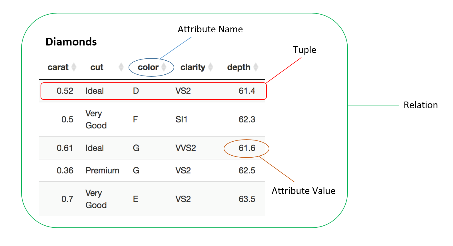
Relational databases and relational query languages follow relational algebra which itself is built upon set theory. There are five fundamental operators in relational algebra, the set union, the set difference, the Cartesian product, the projection, and the selection, of which the only the last two are not borrowed from set theory. These operators act on relations which contain tuples (sets of tuples), as opposed to sets which contain elements (sets of elements). Each relation has a set of attributes from which the values of the tuples derive their domain.
Relational algebra adjusts the operations of set theory with the intention of manipulating tabular data. Additional constraints are placed on set unions and differences whereby they can only be performed on relations which have the same set of attributes. Two relations which have the same set of attributes are said to be union-compatible. The Cartesian product of two relations does not produce a set of 2-tuples containing a tuple from each relation but rather a set of flattened tuples, a concatenation of one tuple from each relation. A projection is a unary operation, one that acts on one relation, which constrains the relation to a subset of its attributes. This is conceptually similar to the projection in linear algebra which is also an idempotent operation, one which applied multiple times gives the same result. The selection operation, also a unary operation, subsets the relation according to a propositional formula (logical statement) whereby each tuple either is either true or false. In a table a projection can be thought of as a column (attribute) subset and a selection as a row (tuple) subset. One more fundamental operation exists which is the unary rename operation. The rename operation takes a specific attribute of a relation and renames it.
First Normal Form
A table was originally proposed by Codd to be in first normal form if and only if all of its attribute domains did not contain any sets as elements. Thus an attribute’s domain can only contain atomic (indivisible) elements and the value of an attribute must be chosen as one and only one element of that domain. This definition of first normal form is problematic however b ecause it requires the indivisibility of elements which is strictly conceptual. There is no rigorous implementation of atomicity. Consider the domain of all phone numbers. The elements themselves are divisible into integer digits and as such the domain can be considered to be a set of sets of digits. One could consider phone numbers to be indivisible (so there is no understanding of them containing digits) but this is both only conceptual in meaning and arbitrarily decided. Chris Date defined a table to be in first normal form if and only if it was a relation. Perhaps a more elegant solution, this definition imposes the following constraints. There is no ordering, either of rows or columns, there exist no duplicate rows, every attribute value is itself one and only one value from the domain, and all columns are regular. The last requirement, all columns are regular, means that each column has a unique name and is visible to every column operator. There can be no ‘special’ columns which function any differently from any other column.
The table below has duplicate rows.
import pandas as pd
import numpy as np
from matplotlib import pyplot as plt
df_1 = pd.DataFrame([[1, 2, 3], [4, 4, 3], [1, 2, 3], [2, 1, 5], [3, 2, 4]], columns=['A', 'B', 'C'])


def plot_database(df_list, title_list, colWidths_list=None, height_scale=2, fig_height=4):
    df_list_len = len(df_list)
    fig, ax = plt.subplots(1, df_list_len, figsize = (8*df_list_len, fig_height))

    # set default column widths
    if colWidths_list is None:
        colWidths_list = []
        for df in df_list:
            colWidths_list.append([0.4 * (df_list_len/len(df.columns))]*len(df.columns))

    # plt.subplots does not return a list if there is only one subplot
    if df_list_len == 1:
        ax = [ax]

    # plot each table in df_list
    header_colours = [[x/256 for x in [173, 216, 230]]]
    for index, df_in in enumerate(df_list):
        col_len = len(df_in.columns)
        table = ax[index].table(cellText=df_in.values,
                                colColours = header_colours*col_len,
                                cellLoc='center',
                                colWidths=colWidths_list[index],
                                colLabels=df_in.columns,
                                loc='center',
                                in_layout=True)
        ax[index].axis('off')
        table.auto_set_font_size(False)
        table.set_fontsize(13)
        table.scale(1, height_scale)
        ax[index].set_title(title_list[index], fontweight='bold')
    plt.show()


plot_database([df_1], ['Table 1'])

To normalise remove the duplicate row..
df_1.drop(2, inplace=True)
plot_database([df_1], ['Table 1'])

Similarly in the case of duplicate columns one can normalise by removing either of the duplicate columns. What if we try to store information via the ordering of the rows? Consider the database below.
df_Clients = pd.DataFrame([[1, 'John Smith'], [2, 'Sarah Perry'], [3, 'Daniel Tan']],
                          columns=['Client ID', 'Client Name'])
df_Children = pd.DataFrame([[1, 'Amy Smith'], [1, 'James Smith'], [1, 'Alex Smith'], [2, 'Luke Perry']],
                          columns=['Client ID', 'Child Name'])

plot_database([df_Clients, df_Children], ['Clients', 'Children'])

Here we have a clients table and a children table. Suppose the intention of the database administrator was to distinguish a given client's children by the order in which they appear. So in the case of the client John Smith, Amy would be the first child, James the second, etc. In practice the relational database managenent system (RDBMS) in use would not be capable of maintaining row order (no RDBMS should ever be able to), but if it did it would violote the orderless priciple of the relational databases. The solution is to add a child number column.
df_Children['Child Number'] = [1, 2, 3, 1]
plot_database([df_Clients, df_Children], ['Clients', 'Children'])

A table is not in first normal form if a row cloumn intersection contains more than one value from the given attribute's domain.
df_customers = pd.DataFrame([['Jess', '0450-345-286'], ['Travis', '0445-932-567'],
                             ['Charlie', '0460-436-937 \n 0460-436-841']], columns=['Name', 'Phone Numbers'])
plot_database([df_customers], ['Customer Phone Numbers'], [[0.2, 0.5]], 3)

To normalise, the repeated element from the domain of phone numbers should be given its own row.
df_customers.loc[df_customers.Name=='Charlie','Phone Numbers'] = '0460-436-937'
df_customers = df_customers.append(pd.DataFrame([['Charlie', '0460-436-841']],
                                   columns=['Name', 'Phone Numbers']), ignore_index=True)
plot_database([df_customers], ['Customer Phone Numbers'], [[0.2, 0.5]], 3)

It would be incorrect to add an additional column for a second phone number.
df_customers.rename(columns={'Phone Numbers': 'Phone Number 1'}, inplace=True)
df_customers.drop(3, inplace=True)
df_customers['Phone Number 2'] = [None, None, '0460-436-841']
plot_database([df_customers], ['Customer Phone Numbers'], [[0.2, 0.5, 0.5]], 3)

Not only is this a case of repeating groups (multiple instances of the same attribute) but there are also null values which violate the need for each row column intersection to be one and only element from the given domain. It is easy to see why adding rows instead of columns is the appropriate way to include multiple elements from a domain.
If a database meets first normal form it was once be said to be normalised. However normalisation has been extended to include many additional and important levels of constraint.
Second Normal Form
Tables have been mathematically described so far as relations. This is true for a given table at a given time but tables can also change and if a table does change so does its associated relation. We intend to alter tables and so it is more accurate to describe them as relational variables, relvars for short. A relvar's domain is all the possible relations it can take on. This is important when discussing the mathematical constraints of higher normal forms.
To be in second normal form a relational variable must be in first normal form and not have any non-prime attributes which are functionally dependent on a strict subset of any candidate key. An attribute is considerd to be a prime attribute if it forms a part of a candidate key and non-prime if it does not from a part of any candidate key. A candidate key defined as a minimal superkey. A superkey is any set of attributes which is unqiue on every tuple for every relation in the relvar's domain. A trivial superkey is the set of all attributes, and a minimal superkey is the smallest subset of those attributes which still remains a superkey.
Thus given a compound key (one which consists of two or more attributes) then any attribute not a part of the compound key which is functionally dependant on any part of the key should also be functionally dependant on the whole key.
df_schools = pd.DataFrame([['A. Valley', 100, 'Hopkins Primary', 'Paul Smith'],
                           ['A. Valley', 101, 'Bellevue High' ,'Paul Smith'],
                           ['Orange County', 26, 'Venture Collage', 'John Jones'],
                           ['Orange County', 100, 'Santa Monica High', 'John Jones']],
                         columns = ['District', 'School Id', 'School Name', 'Superintendent'])
plot_database([df_schools], ['Schools'], [[0.4, 0.2, 0.4, 0.4]])

Above in the Schools table the District and School Id attributes give rise to a candidate key. For any district there is a school ID for all schools in the district. Schools in different districts may have the same school ID. Given that School Id and District make a candidate key we require any non-prime attributes to be functionally dependent on the whole key if they depend on any of it. School Name and Superintendent are both non-prime attributes because they do not form part of a candidate key. One might consider Superintendent and School Id to form a candidate key but two school districts could have the same superintendent. District to Superintendent is not necessarily a one-to-one relationship. In this case we have that Superintendent functionally depends on District but not School Id.
To remedy this we can create a Superintendendents table.
df_superintendents = pd.DataFrame(np.transpose(np.array([df_schools['District'],
                                                         df_schools['Superintendent']])),
                                 columns=['District', 'Superintendent'])
df_schools.drop('Superintendent', axis=1, inplace=True)
plot_database([df_schools, df_superintendents], ['Schools', 'Superintendents'], [[0.4, 0.2, 0.4], [0.4, 0.4]])

The Superintedents table is actually just a column subset of the original Schools table. It is the projection of Schools onto the attribute set {District, Superintenedents}. Similarly the schools table is a new relvar, the projection of Schools onto the attribute set {District, School Id, School Name}. Here we have removed a funtional redundancy by taking two projections. This process lies at the core of normalisation. Much of normalisation consists of removing redundancies by taking projections.
Third Normal Form
To be in third normal form a relvar must be in second normal form and all of its attributes must all be functionally dependent on the primary key. A primary key is a key chosen from amoung the candidate keys to uniquely specify all the tuples in the relvar. This requires that there be no transient dependencies in the relvar. The essence of achieving third normal form is removing transient functional dependencies.
Consider the patients table below.
df_patients = pd.DataFrame([[1, 'John Smith', 'Samuel Tan', '0472-3450-293'],
                            [2, 'Alex Anderson', 'Samuel Tan', '0472-3450-293'],
                            [3, 'Gerald Rutherford', 'Sasha Ling', '0420-459-533']],
                            columns=['Patient ID', 'Name', 'Doctor', "Doctor's Phone Number"])
plot_database([df_patients], ['Patients'], [[0.2, 0.4, 0.4, 0.5]])

The primary key is Patient ID and both Name and Doctor are functionally dependent on Patient ID. Doctor's Phone Number is only functionally dependent on Doctor. Thus Doctor's Phone Number is transiently dependent on Patient ID. To remove the transient dependency we can create a Doctors table.
df_doctors = pd.DataFrame(np.transpose(np.array([df_patients['Doctor'],
                                                 df_patients["Doctor's Phone Number"]])),
                                 columns=['Doctor', "Doctor's Phone Number"])
df_doctors.drop(1, axis=0, inplace=True)
df_patients.drop("Doctor's Phone Number", axis=1, inplace=True)
plot_database([df_patients, df_doctors], ['Patients', 'Doctors'], [[0.2, 0.4, 0.4], [0.4, 0.5]])

Both the new Patients table and the Doctors table are results of projects of the original Patients table onto subsets of its attributes. A transitive functional dependency has been removed via projections.
Elementary Key Normal Form
A key K is considered an elementary key if there exists another attribute which has a non-trivial and irreducible functional dependency on K. Any functional dependency of this kind is called an elementary fucntional dependency. If all of a relvar's elementary functional dependencies begin at whole keys or end at an elementary key attribute the relvar is said to be in elementary key normal form (EKNF). Given an elementary functional dependency K --> A in a relvar R, EKNF requires either K be a an elementary key or A be a part of an elementary key.
Elementary key normal form is not discussed often because it does not constitute a major milestone in database normalisation. The proceeding form, Boyce-Codd normal form (BCNF) is much more significant. However, it is possible for a relvar in third normal form to be unable to meet BCNF. It is in this corner case EKNF takes on a unqiue significance.
If a relvar has overlapping compound keys it fails to meet elementary key normal form. If the same relvar has functional dependencies of the form {AB --> C, C --> B} then it consistitues an example of the previously alluded to corner case. In such a situtation the relvar cannot be losslessly decomposed to meet BCNF and the highest normal form achievable for the relvar remains EKNF. A decomposition is lossless if and only if natural joins will always return the original relvar.
df_person = pd.DataFrame([['James', 'Restaurant', 'Chili Burgers'],
                          ['James', 'Hairdresser', 'Best Cuts'],
                          ['Sam', 'Bookshop', 'Bookland'],
                          ['Alex', 'Restaurant', 'Jumbo Kebabs'],
                          ['Alex', 'Hairdresser', 'Best Cuts']],
                         columns=['Person', 'Shop Type', 'Nearest Shop'])

plot_database([df_person], ['Nearest Shops by Type'], [[0.3, 0.4, 0.4]])

The table above records the nearest shop of each type for each person. Given both the Person attribute and Shop Type attribute we can uniquely indentify the nearest shop of that type. This implies the function dependency of Nearest Shop on Person and Shop Type. For a given person there is only one Nearest Shop of a certian Shop Type thus Person and Nearest Shop uniquely determines Shope Type. Here we have two overlapping compound keys, Person and Shop Type, and Person and Nearest Shop. This means the relvar is not in EKNF.
It is also true that given the Nearest Shop we have the Shop Type. So there exists a functional dependency of the form {AB --> C, C --> B}, where A = Person, B = Shop Type, and C = Nearest Shop. Thus the relvar can never be losslessly decomposed to meet BCNF. Taking projections, Person and Nearest Shop, and Shop and Shop Type results into two relvars which meet BCNF. However recomposition with a naturual join does not guarentee the funcitonal dependency, Person and Shop Type implies Shop, will be respected.
The following lossless decomposition respects EKNF.
df_shop = pd.DataFrame(np.transpose(np.array([df_person['Nearest Shop'],
                                                 df_person['Shop Type']])),
                                 columns=['Shop', 'Shop Type'])
df_shop = df_shop.drop(4)
plot_database([df_person, df_shop], ['Nearest Shops by Type', 'Shops'], [[0.3, 0.4, 0.4], [0.4, 0.4]])

The Nearest Shop attribute was renamed to Shop in the Shops table and duplicate tuples were removed. If Nearest Shop is a foreign key then the functional dependency, Nearest Shop implies Shop Type, no longer exists in the Nearest Shops by Type table. Instead Shop Type can be infered from the foreign key Nearest Shop through the Shops table. Thus we no longer have any non-elementery functional dependencies.
Boyce-Codd Normal Form
As well as being in third normal form, Boyce-Codd normal form requires all functional dependencies to be either trivial dependencies or dependencies on a superkey. If a relvar in third normal form does not have overlapping compound keys it is necessarily in BCNF. To achieve BCNF relvars with overlapping composite keys are losslessly decomposed with projections.
df_enrol = pd.DataFrame([[1, 'M210', 'Real Analysis'],
                         [1, 'M212', 'Algebra and Number Theory'],
                         [2, 'M212', 'Real Analysis']],
                        columns=['Student ID', 'Course ID', 'Course Name'])
plot_database([df_enrol], ['Enrollments'], [[0.2, 0.2, 0.5]])

In the enrollments table both Course ID and Course Name are unique and as such both paired with Student ID form overlapping compound keys. Taking projections of attribute subsets, Student ID and Course ID, and Course ID and Course Name we have losslessly decomposed Enrollments to meet BCNF.
df_courses = pd.DataFrame(np.transpose(np.array([df_enrol['Course ID'], df_enrol['Course Name']])),
                          columns=['Course ID', 'Course Name'])
df_enrol = pd.DataFrame(np.transpose(np.array([df_enrol['Student ID'], df_enrol['Course ID']])),
                          columns=['Student ID', 'Course ID'])
plot_database([df_enrol, df_courses], ['Enrollments', 'Courses'], [[0.2, 0.2], [0.2, 0.6]])

Now all non-trivial functional dependencies are on superkeys.
Fourth Normal Form
The fourth normal form is concerned with removing mutlivalued dependecies. A multivalued dependency is a binary join dependency. A relvar is in fourth normal form if and only if all of its non-trivial multivalued dependencies are dependencies on a superkey.
df_friends = pd.DataFrame([['James', 'Rock Climbing', 'Cooking'],
                           ['James', 'Rock Climbing', 'Videogames'],
                           ['Luke', 'Rock Climbing', 'Dumpster Diving'],
                           ['Luke', 'Hockey', 'Dupster Diving'],
                           ['Paula', 'Horse Riding', 'Cooking'],
                           ['Paula', 'Running', 'Cooking'],
                           ['Paula', 'Horse Riding', 'Knitting'],
                           ['Paula', 'Running', 'Knitting']],
                         columns=['Name', 'Sport', 'Hobby'])

plot_database([df_friends], ['Friends'], [[0.3, 0.4, 0.4]])

The above table is of friends and their sports and hobbies. The only superkey is the trivial superkey of all attributes. There is a multivalued dependecy from Name to Sport and Hobby. Both Sport and Hobby depend on Name but they are independent of each other. This means if we want to add another hobby for a friend we must add tuples for every sport. This redundancy exposes the database to insert anomolies. There is no way of verifying all sports have been matched with the new hobby.
df_sports = df_friends[['Name', 'Sport']].copy()
df_sports.drop_duplicates(inplace=True)
df_hobbies = df_friends[['Name', 'Hobby']].copy()
df_hobbies.drop_duplicates(inplace=True)

plot_database([df_sports, df_hobbies], ['Sports', 'Hobbies'])

By decomposing the Friends table into two projections, Sports and Hobbies, the database is now in fourth normal form. If a new hobby is added to a friend only one row needs to be inserted thus removing the previous redundancy.
Fifth Normal Form
A relvar is in fifth normal form if and only if all join dependencies present are comprised entirely of candidate keys. Given a join dependency {$X_{1}$, $X_{2}$, ..., $X_{n}$} where each X is a subset of attributes, the join dependency is comprised entirely of candidate keys if each X is a candidate key. It is rarely the case that a relvar in fourth normal form is not also in fifth noraml form. It is the presence of real world sematic relationships between attribues which prevents a fourth normal form table from meeting fifth normal form constraints. The table below explores this possibility.
df_skills = pd.DataFrame([['Smith', 'A', 'Java'],
                          ['Smith', 'A', 'HTML'],
                          ['Smith', 'B', 'Java'],
                          ['Smith', 'C', 'HTML'],
                          ['Jones', 'C', 'Python'],
                          ['Jones', 'B', 'TypeScript'],
                          ['Anderson', 'A', 'Java']],
                         columns = ['Employee', 'Project', 'Skill'])

plot_database([df_skills], ['Employee Project Skills'], [[0.3, 0.2, 0.3]])

Note the Employee Project Skills only considers skills which are used on projects and does not consider a skill an employee has if it is not used on a project. The table has one superkey, the trivial superkey, and is in fourth normal form because there are no binary join dependencies. If there are no rules on which skills an employees use on a given project the table is in fifth normal form. Then there exists no lossless decomposition and the table in its current state is the only way to correctly model the situation. Suppose however that if a certain skill is used on a given project and an employee which posses the same skill is also working on the project then that employee will always use the givin skill on the project. This real world semantic relationship creates a ternary join dependency of the form {$X_{1}$, $X_{2}$, $X_{3}$,} where $X_{1}$ = {Employee, Project}, $X_{2}$ = {Project, Skill}, and $X_{3}$ = {Employee, Skill}. In order to meet fifth normal form it is now necessary to decompose the relvar into the three aforementioned projections
df_employee_projs = df_skills[['Employee', 'Project']].copy()
df_employee_projs.drop_duplicates(inplace=True)
df_employee_skills = df_skills[['Employee', 'Skill']].copy()
df_employee_skills.drop_duplicates(inplace=True)
df_proj_skills = df_skills[['Project', 'Skill']].copy()
df_proj_skills.drop_duplicates(inplace=True)

plot_database([df_employee_projs, df_employee_skills, df_proj_skills],
              ['Employee Projects', 'Employee Skills', 'Project Skills'], [[0.5]*2]*3, 2.5, 4)

The above decomposition is lossless given every employee working on a project who has a skill that can be used on the project does use the skill on the project. The databse now meets fifth normal form. Before whenever an additional employee is added to a project updating the table required adding rows for every skill used by the employee and project. Now only one row needs to be added the the Employee Projects table.
Domain Key Normal Form
A relvar is in domain key normal form (DKNF) if and only if all constraints present are logical consequences of the relvar's keys and attribute domains. For most relational databases DKNF is the penultimate goal, which when accomplished prevents the database from becoming inconsistant via insert, update, and delete anomolies. Logical consequences of keys and domians are enforced by the RDBMS, such as being unable to insert a str type in a float type coloumn or update a table with a row that violates a unique key constraint.
df_purchases = pd.DataFrame([[1,'Member Non-Bulk Buyer', 26.55], [2, 'Non-Member Bulk Buyer', 65.00],
                                 [3, 'Non-Member Non-Bulk Buyer', 10.00], [4, 'Member Bulk Buyer', 73.40],
                                 [5, 'Non-Member Bulk Buyer', 55.50]],
                           columns=['Transaction ID', 'Buyer Type', 'Cost'])

plot_database([df_purchases], ['Purchases'], [[0.3, 0.5, 0.2]])

In the purchases table above consider the possible relationship between Cost and Member. Any purchase of \$50.00 or over classifies a buyer as a Bulk Buyer. This constraint on Buyer Type by Cost violates DKNF because the constriant is neither a consequence of the domains of Cost or Member or of the key Transaction ID. Given Cost one can know the if the buyer is a bulk buyer or not, but Cost does not determine if the buyer is a member. Note the table is in fifth normal form becuase the only non-trivial join dependency is on the candidate key Transaction ID. We can create two new attributes by splitting Buyer Type's domain.
df_purchases_new = pd.DataFrame([[1,'Yes', 26.55], [2, 'No', 65.00], [3, 'No', 10.00],
                             [4, 'Yes', 73.40], [5, 'No', 55.50]],
                            columns=['Transaction ID', 'Member', 'Cost'])
df_buyer_type = pd.DataFrame([['Non-Bulk Buyer', 00.00, 49.99], ['Bulk Buyer', 50.00, 999999.99]],
                            columns=['Type', 'Minimum', 'Maximum'])
plot_database([df_purchases_new, df_buyer_type], ['Purchases', 'Buyer Type'], [[0.3, 0.2, 0.2], [0.4, 0.2, 0.2]])

Given a buying limit of 1 million dollars the database now conforms to DKNF. No information is lost and the constraint between Buyer Type and Cost is clearly laid out in the Buyer Type table.
Sixth Normal Form
A relvar is in sixth normal form if and only if there exist no trivial join dependencies on the relvar. In essence this reduces all tables into all combinations of the candidate keys and one other attribute.
df_people_2 =  pd.DataFrame([[1, 'Sarah', 'Sanders', 26], [2, 'James', 'Smith', 14],
                             [3, 'John', 'Smith', 34], [4, 'Alex', 'Perry', 28],
                             [5, 'Lily', 'Chin', 44], [6, 'Amy', 'Thompson', 23]],
                            columns=['Person ID', 'First Name', 'Last Name', "Age"])

plot_database([df_people_2], ['People'], [[0.2, 0.3, 0.3, 0.2]])

The People table above is in DKNF because there are no contraints present other than key and domain constraints. There is one candidate key, Person ID. To put this table in sixth normal form we can decompose the table into candidate key and attribute pairs.
df_first_name = df_people_2[['Person ID', 'First Name']].copy()
df_last_name = df_people_2[['Person ID', 'Last Name']].copy()
df_age = df_people_2[['Person ID', 'Age']].copy()

plot_database([df_first_name, df_last_name, df_age], ['First Name', 'Last Name', 'Age'],
              [[0.2, 0.3], [0.2, 0.3], [0.2, 0.2]])

The purpose of such a table decomposition, and thus sixth normal form, is usually significant only when considering temporal relational databases. In temporal relational databases data is exists temporally. That means depending on time data may take on different values. In such a case it can be useful to have a database in sixth normal form.
Conclusion
Although many of the examples used were somewhat contrived they capture the essence of each normal form. In practice many databases may not need to meet DKNF if data integrity is not the highest priority. When data integrity is of the utmost importance it is necessary to constrain the database to DKNF.