Sugarcane Polygons
Introduction
Inspired by the Melbourne 2019 Datathon, this project consists of a python library for working with satillite images, featuring pixel classification, image processing, and polygon masks. Here we will take a journey, starting with raw satillite images from the European Space Agency's (ESA) SENTINEL program to through the creation of polygon objects which mask for sugarcane. Sugarcane is a significant Australian industry, coming in as Australia's second largest crop export. We will examine land in Proserpine, Queensland, one of Australia's largest surgarcane producing regions.
Sentinel Data
The Sentinel 1 and 2 (S1 and S2) satilite missions provide radar and optical imaging respectively, and their data is free to download at https://sentinel.esa.int/web/sentinel/home. The data is provided as Sentinel products, containing various information, including several wavelengths (bands), images taken at different solar angles, and geolocation data. We will need SNAP, which ESA's dedicated program for working with Sentinel products.
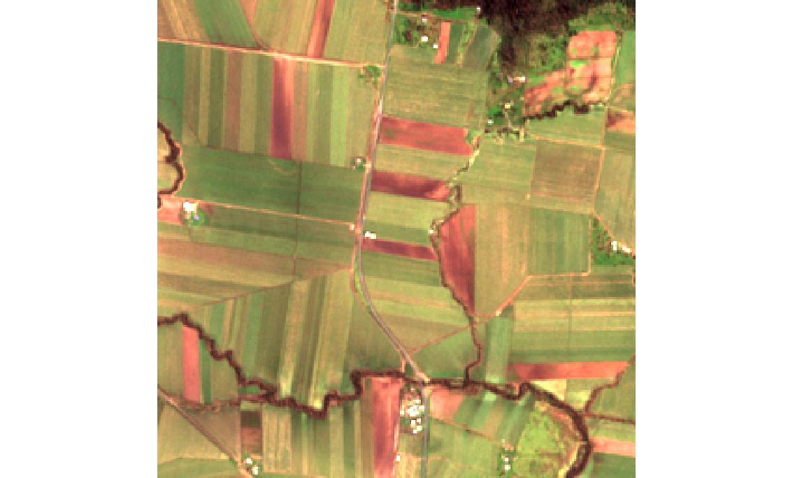
Below we have a subset of the Proserpine region, in optical Bands 4, 3, and 2, which correspond to the natural RGB wavelengths (665 nm, 560 nm, and 665 nm respectively).
from IPython.display import HTML
HTML("""
    <img alt="optical" source src="optical_unprocessed.png">
    </img>
""")
As well as optical data we also have two bands of radar data, Amplitude_VH, and Amplitude_VV (VH, and VV for short). These bands correspond to the horizontal and vertical polarisation of radar radiation both sent and recieved. Differently oriented radiation reflect disproportionately off differing surfaces, and as such these bands provide useful a tool for distinguishing vegetation. We can map these two bands to RG for visualization.
from IPython.display import HTML
HTML("""
    <img alt="optical" source src="radar_unprocessed.png">
    </img>
""")
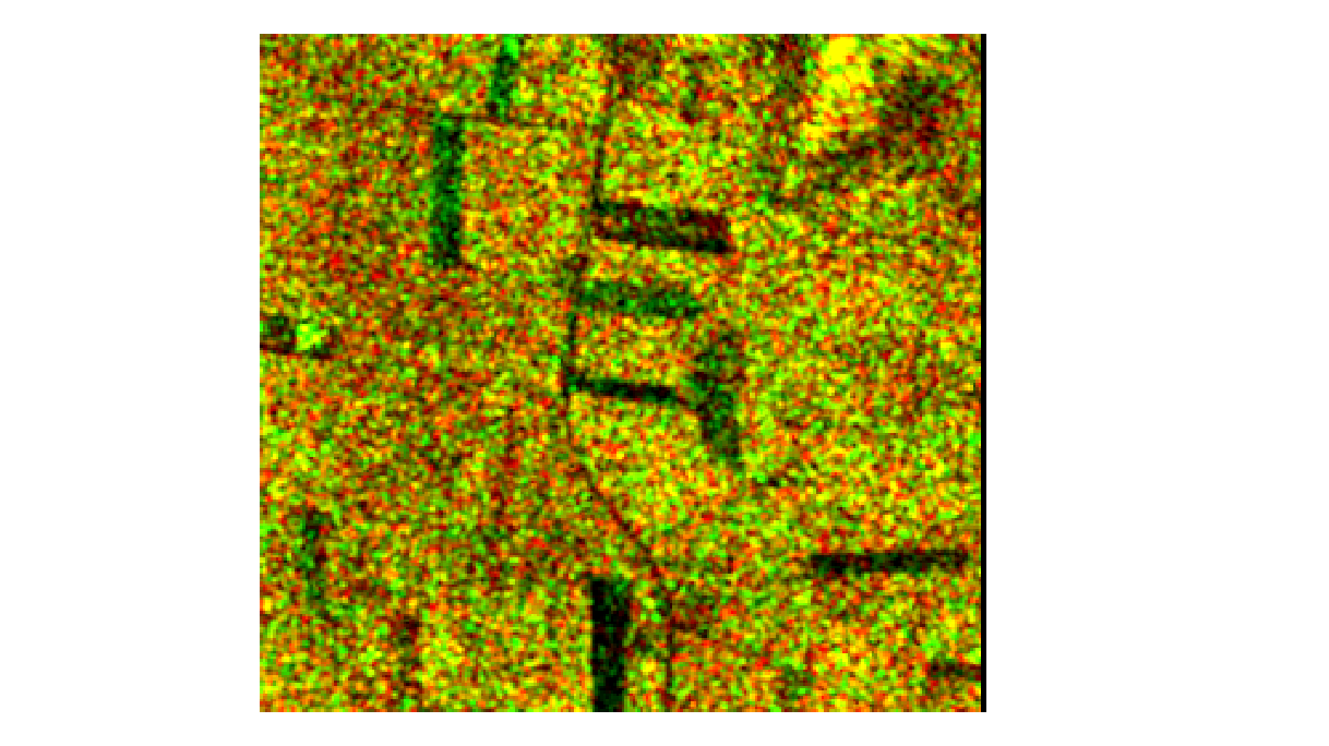
It is noticeable how well intensity correlates with the presence of vegetation. Where crops have been recently harvested and are yet to be replanted there are dark patches.
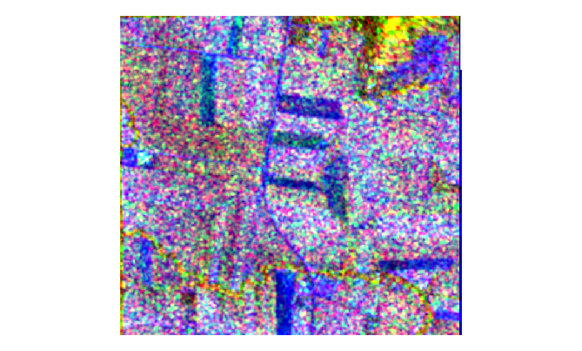
Now working with satellite data requires some important pre-processing steps. We can't combine these two images just yet. First we must reproject, a geo-coordinate transformation to form an accurate two-dimensional image from what is technically three dimensional data (the earth's surface is curved) and to ensure both the optical and radar data align properly. Next, we perform a terrain correction to account for differences in elevation, and then resample, for differences in resolution across bands. Finally we can subset, choosing only the region and bands we want to consider. SNAP can now merge the two images with a collocation operation. The resultant image mapped to RGB does not reveal much, but it is definitely colourful!
from IPython.display import HTML
HTML("""
    <img alt="collocate_RGB" source src="collocate_RGB.png">
    </img>
""")
SNAP will export the collocate object as a tiff file which we process manipulate as a multi-dimensional array. It will be important to recover the optical portion from the tiff file as an RGB image to visualize our starting point. In the 'preprocessing' module we have the fucntion 'color_correction'.
import imageio

def color_correction(path):
    """Takes tiff product and produces optical image array in RGB."""

    image1 = imageio.imread('RF_input/{}.tif'.format(path))
    optical = image1[2:5, :, :]

    # scale optical portion to dl (some tiff files have the optical data in dl 0-1, and others the raw 0-10000)
    if np.nanmean(optical) > 1:
        op = 1
    else:
        op = 0
    optical = np.transpose(optical, [1, 2, 0]) / (10000*op + (1 - op))
    optical = np.flip(optical, axis=2)

    # get 95th and 5th percentiles
    max_colors = np.array([np.nanpercentile(optical[:, :, 0], 95), np.nanpercentile(optical[:, :, 1], 95),
                           np.nanpercentile(optical[:, :, 2], 95)])
    min_colors = np.array([np.nanpercentile(optical[:, :, 0], 5), np.nanpercentile(optical[:, :, 1], 5),
                           np.nanpercentile(optical[:, :, 2], 5)])

    # set NANs to 0
    optical = np.nan_to_num(optical, nan=0)

    # clip values to 95th and 5th percentile
    optical[:, :, 0] = np.clip(optical[:, :, 0], min_colors[0], max_colors[0])
    optical[:, :, 1] = np.clip(optical[:, :, 1], min_colors[1], max_colors[1])
    optical[:, :, 2] = np.clip(optical[:, :, 2], min_colors[2], max_colors[2])

    # scale to 0 - 255 RGB
    scalar_colors = 255 / (max_colors - min_colors)
    optical_colored = np.rint((optical - min_colors) * scalar_colors).astype('int')

    return optical_colored
import preprocessing as prep
from matplotlib import pyplot as plt
fig, ax = plt.subplots(1, 1, figsize=(12.8,9.6))
ax.imshow(prep.color_correction('collocate'))

Training Data
To create training data for our machine learning algorithms we are going to need to select large quanties of pixels and classify them manually. Pixel Annotation Tool is a program designed essentially for that purpose. We can select different colors and brushes and mark our image accordinly to produce a mask image with different RGB values for each color.
from IPython.display import HTML
HTML("""
    <img alt="collocate_Mask" source src="collocate_mask.png">
    </img>
""")

The output image has RGB greyscale values denoting each classification, such as (21, 21, 21) for sugarcane. There are six different classifications, sugarcane, dirt, building, forest, water, and other vegetation. For the sake of variety and sample size another image from the Proserpine region has masked with training pixels.
from IPython.display import HTML
HTML("""
    <img alt="collocate2_Mask" source src="collocate2_mask.png">
    </img>
""")

Now we can process both the mask files and the tiff file together to produce training data as a pandas dataframe. The tiff data needs to be rescaled to dimensionless units (0 - 1). The position and order of the training pixels are unimportant, just the feature values, so the two dimensional position data of the pixels can be flattened to one dimension. This is accomplished with the 'data_prep' function in the 'preprocessing' module.
def data_prep(path):
    """prepares data for ML input"""

    # read and transpose
    image1 = imageio.imread('RF_input/{}.tif'.format(path))
    image1 = np.transpose(image1, [1, 2, 0])

    # scale optical portion to dl (some tiff files have the optical data in dl 0-1, and others the raw 0-10000)
    # and reorder to RGB
    optical = image1[:, :, 2:5]
    if np.nanmean(optical) > 1:
        op = 1
    else:
        op = 0
    optical = optical / (10000*op + (1 - op))
    optical = np.flip(optical, axis=2)

    # scale radar portion to dl (some tiff files have the radar data in dl 0-1, and others the raw 0-10000)
    radar = image1[:, :, 0:2]
    if np.nanmean(radar) > 1:
        ra = 1
    else:
        ra = 0
    radar = radar / (10000 * ra + (1 - op))

    # combine radar and optical and flatten to 1-D
    collocate = np.concatenate((optical, radar), axis=2)
    shape = collocate.shape[0] * collocate.shape[1]
    collocate_flattened = np.reshape(collocate, (shape, 5))

    return collocate_flattened
The flattened pixel data is combined with the classification from the mask image and structured as a dataframe.
def mask_data(collocate_flattened, path):
    """masks training data"""

    # read mask array, change its shape, and flatten it
    mask = imageio.imread('RF_input/masks/{}_mask.png'.format(path), 'png')
    shape = mask.shape[0] * mask.shape[1]
    mask_flattened = np.reshape(mask, (shape, 3))

    # collapse redundant values along the mask RGB dimension to one scalar value, e.g. [4, 4, 4] --> [4]
    mask_collapsed = []
    for mask_value in mask_flattened[:, 0]:
        mask_collapsed.append(mask_value)
    mask_collapsed = np.array(mask_collapsed)

    # remove elements in the collocate and mask arrays which have no mask value associated with it
    collocate_masked = collocate_flattened[~(mask_collapsed == 0)]
    mask_collapsed = np.expand_dims(mask_collapsed[~(mask_collapsed == 0)], axis=1)

    # create dataframe, remove NaNs, and substitute mask values with more appropriate ML values
    data1 = np.concatenate((collocate_masked, mask_collapsed), axis=1)
    collocate_train_df = pd.DataFrame(data=data1, columns=['R', 'G', 'B', 'VH', 'VV', 'Mask'])
    collocate_train_df = collocate_train_df.dropna(axis=0, how='any')
    collocate_train_df = collocate_train_df.replace({'Mask': {21: 1, 8: 2, 24: 3, 19: 4, 30: 5, 25: 6}})
    collocate_train_df = collocate_train_df.astype(np.float64)

    return collocate_train_df


def training_data(path):
    """call data_prep and mask_data"""

    return mask_data(data_prep(path), path)
import preprocessing as prep
training_df = prep.training_data('collocate')
training_df[0:10]
Pandas dataframes are useful but what if we want to progressively add more training data? We are going to need a database to provide permanency and reusability for our training data. To prevent duplicate training data being added to the database a key is created for each pixel. The key will include information pertaining to the position of the pixel in the image and the image's file name. Thus each pixel from each image will have a unique key and we can set a unique constraint for the key column in our table. Here I have used Microsoft's SQL Server (MSSQL).
CREATE TABLE training_data (
    R FLOAT NOT NULL,
    G FLOAT NOT NULL,
    B FLOAT NOT NULL,
    VH FLOAT NOT NULL,
    VV FLOAT NOT NULL,
    mask INT NOT NULL,
    pixel_id VARCHAR(50) UNIQUE,
);
To catch the error thrown when duplicate data is added to the table the follwoing stored procudure is used.
CREATE PROCEDURE usp_GetErrorInfo
AS
SELECT
    ERROR_NUMBER() AS ErrorNumber
    ,ERROR_SEVERITY() AS ErrorSeverity
    ,ERROR_STATE() AS ErrorState
    ,ERROR_PROCEDURE() AS ErrorProcedure
    ,ERROR_LINE() AS ErrorLine
    ,ERROR_MESSAGE() AS ErrorMessage;
GO
Now we can take the dataframe and the parent image filename, create the unique pixel key, restructure the data for insertion into the database, and add it to the 'training_data' table. In the 'database' module we have the function 'add_training_data'.
import pymssql
import numpy as np

def add_training_data(data, path):
    """adds training data to training database"""

    # convert numpy array into python nested list
    values_list = [tuple(elem) for elem in list(data.values)]

    # create keys for each pixel as a string of file name + pixel number
    key_list = [path + '_{}'.format(number) for number in range(1, data.values.shape[0] + 1)]

    # combine keys and data into a python nested list with both string and float data types
    data_and_key = [sublist + (elem,) for sublist, elem in zip(values_list, key_list)]

    # connect to database
    connection = pymssql.connect(host='localhost',  user='sa', password='password_sa1', database='TestDB')
    cursor = connection.cursor()

    # insert data into database and return any errors
    cursor.executemany("""
        BEGIN TRY
            INSERT INTO training_data VALUES (%s, %s, %s, %s, %s, %s, %s);
        END TRY
        BEGIN CATCH
            EXECUTE usp_GetErrorInfo;
        END CATCH;
         """, data_and_key
                       )

    # fetch any error if it exists
    try:
        error = cursor.fetchall()
    except pymssql.OperationalError:
        error = None

    # if there was a 'UNIQUE KEY constraint' error in the sequel query print the specified message, if there was any
    # other error print any relevant information, otherwise pass
    if not(error is None):
        if error[0][0] == 2627:
            print('You have tried to add duplicate keys to the database. This means the image and its'
                  ' associated pixels are already in the database.')
        else:
            print(error)

    # commit any transactions and close
    connection.commit()
    connection.close()

    return None
database.add_training_data(prep.training_data('collocate'), 'collocate')
database.add_training_data(prep.training_data('collocate2'), 'collocate2')
Examine the top 10 rows of our training data.
SELECT TOP 10 * FROM training_data
R              G              B              VH             VV             mask           pixel_id
-------------- -------------- -------------- -------------- -------------- -------------- --------------------------------------------------
        0.0473   6.6299997E-2   8.0499999E-2   1.0106611E-2   2.0517068E-2            2.0 collocate_1
  4.9800001E-2   7.0100002E-2         0.0814     0.01078363   1.8041631E-2            2.0 collocate_2
  4.9800001E-2   7.0100002E-2         0.0814   1.6678311E-2   2.2439957E-2            2.0 collocate_3
         0.048   6.9499999E-2   8.2500003E-2     0.02038555   2.0471895E-2            2.0 collocate_4
        0.0504         0.0682   8.1500001E-2   3.0804858E-2   2.4607506E-2            2.0 collocate_5
  5.4400001E-2   7.3600002E-2   8.4700003E-2   3.6135249E-2     0.02377356            2.0 collocate_6
  5.9500001E-2   7.7600002E-2   8.8500001E-2   3.3722445E-2   2.3607958E-2            2.0 collocate_7
  6.4400002E-2   8.1299998E-2   8.7300003E-2   2.8583148E-2   2.1298056E-2            2.0 collocate_8
         0.055         0.0766   8.4399998E-2   2.0565461E-2   2.3377135E-2            2.0 collocate_9
        0.0557   7.6399997E-2   8.5500002E-2   1.5100362E-2   2.5102066E-2            2.0 collocate_10
SELECT COUNT(*) FROM training_data
-----------
      28040
Between both tranining data images there are over 28,000 classified pixels of six different labels.
Classification
Below is the function in the 'database' module for fetching the training data as a pandas dataframe.
def fetch_training_data():
    """Return all training data in the database"""

    # connect to database
    connection = pymssql.connect(host='localhost',  user='sa', password='password_sa1', database='TestDB')
    cursor = connection.cursor()

    # select all from training_data
    cursor.execute('SELECT * FROM training_data')

    # fetch results and assign to pandas dataframe
    training_data_df = pd.DataFrame(cursor.fetchall(), columns=['R', 'G', 'B', 'VH', 'VV', 'Mask', 'Pixel_id'])

    return training_data_df
We will use sklearn's ML algorithms for classification. The 'classifier' module contains the 'ClassifierBuilder' class. A class which allows us to streamline obtaining the training data, splitting it into train and test sets, and testing common classifiers.
import classifier

clf_build_1 = classifier.ClassifierBuilder()
clf_build_1.rf_classifier()
clf_build_1.sgd_classifier()
clf_build_1.svm_classifier()
Above are the training accuracy scores for a Random Forest, a Stochastic Gradient Descent, and a Support Vector Machine classifier. The hyperparamters of the classifiers have been previosly tuned and set as default in the 'ClassifierBuilder' class. Let us use the Random Forest classifier and save the prediction.
clf_build_1.rf_classifier()
prediction = clf_build_1.predict()
np.savetxt('prediction.csv', clf_build_1.prediction)
The 'postprocessing' module consists of the 'ProcessedPrediction' class which allows us to view the raw classifier output as well as process the resultant image to remove noise, isolated pixels, etc. The first two methods 'multi_label_to_image' and 'binary_label_to_image' show us the classification for all labels and also the binary non-sugarcane / sugarcane classifition.
import postprocessing as postp
import numpy as np
from matplotlib import pyplot as plt

prediction = np.genfromtxt('prediction.csv', delimiter=',')
mask_1 = postp.ProcessedPrediction(prediction)
mask_1.postpro_level_0()
mask_1.multi_label_to_image()
mask_1.binary_label_to_image()
fig, ax = plt.subplots(2, 1, constrained_layout=True, figsize=(25.6,19.2))
ax[1].imshow(mask_1.binary_label_image)
ax[0].imshow(mask_1.multi_label_image)
plt.show()

Mask Processing
For the creation of a sugarcane mask we are interested only in the binary classification. There is plenty proccesing we are going to have to do to the raw ML output to improve the quality of out mask. Let us start by building an isolated pixel remover. This function will examine the pixels around a chosen central pixel in a given radius. The given pixel's binary value can then be altered if the ratio of like-valued neighboring pixels is too low, thus removing isolated pixels.
def isolated_pixel_remover(self, r=0):
    """Removes isolated pixels under limiting conditions with a specified radius"""

    # setup window with all ones and total_sum with all zeros
    diameter = 2*r + 1
    window = np.ones((diameter, diameter))
    total_sum = np.zeros(self.processed.shape)
    arr_out = self.processed.copy()

    # loop through window
    for (x, y), weight in np.ndenumerate(window):
        view_in, view_out = routines.view(y - 1, x - 1, self.processed.shape)
        total_sum[view_out] += self.processed[view_in]

    # If the ratio of 1s in the window is less than 0.2 set change central pixel to a 0
    arr_out[total_sum < ((diameter**2) * 0.2)] = 0

    # If the ratio of 1s in the window is greater than 0.8 change the central pixel to a 1
    arr_out[total_sum > ((diameter**2) * 0.8)] = 1

    return arr_out
It is important for this algorithm to be fast. A simple for loop through each pixel will be very slow especially as we already have over 67500 pixels in this image alone. Above, we have made use of a sliding window technique which creates arrays of identical shape, but offset, for a given viewing window. For example, for a 3 x 3 window 8 new arrays will be created of which each map the value of one surrounding pixel to the position of the central pixel. If we want the sum of all the values surrounding each pixel in an array we can simply add up those 8 arrays.
def postpro_level_0(self):
    """group all classified pixels as sugarcane or non-sugarcane and reshape to 2-D numpy array"""

    # dictionary associating ML values with sugarcane or non-sugarcane
    color_dict = {1: 1, 2: 0, 3: 0, 4: 0, 5: 0, 6: 0}

    # covert ML values to RGB color
    predict_binary = [color_dict[key] for key in self.prediction]

    # reshape 1-D array into 2-D array
    predict_reshaped = np.reshape(np.array(predict_binary), (255, 273))

    self.processed = predict_reshaped

def postpro_level_1(self):
    """upgrades/downgrades postprocessing to level 1 by removing isolated pixels"""

    self.postpro_level_0()
    self.processed = self.isolated_pixel_remover(2)

def postpro_level_2(self):
    """upgrades/downgrades postprocessing to level 2 by removing isolated pixels"""

    self.postpro_level_1()
    self.processed = self.isolated_pixel_remover(1)
from matplotlib import patches

mask_1.postpro_level_2()
postpro_lvl2 = mask_1.processed
fig, ax = plt.subplots(1, 1, constrained_layout=True, figsize=(12.8,9.6))
palette = np.array([[210, 180, 140],
                    [0,   128,   0]])
patches_list = [patches.Patch(color='#d2b48c'), patches.Patch(color='#008000')]
plt.legend(handles=patches_list, labels=['non-sugarcane', 'sugarcane'], bbox_to_anchor=(1.05, 1),
           loc=2, borderaxespad=0., fontsize='x-large')
ax.imshow(palette[postpro_lvl2], interpolation='nearest')
plt.show()

After two levels of processing our image has significantly reduced noise, however we are not going to want to polygons with this level of precision. In reality sugarcane is distributed amoung fields which show up as homogenous large grouping of sugarcane. There is likely no field where sugarcane has been predicted sporadictly, such as the bottom right of image, around coordinates (200-250, 200-250). A more aggressive strategy is needed before we try to locate bounding polygon coordinates.
There are two field edge flattening algorithms in the 'ProcessedPrediction' class, 'edge_flatten' and 'edge_flatten_2'. The first eliminates sugarcane pixels which have in a one pixel radius, along a cardinal dimension, have no neighboring sugarcane pixels.
def edge_flatten(self, r=0):
    """Removes pixels (within the specified radius) with zero like neighboring pixels along one of the two
     cardinal dimensions, e.g. [[0, 1, 1],
                                [0, 1, 0],
                                [0, 0, 0]
    has zero like neighboring pixels along the right-left dimension ([0, 1, 0]) and will be removed"""

    # setup
    total_sum_2 = np.zeros(self.processed.shape)
    total_sum_1 = np.zeros(self.processed.shape)
    arr_out = self.processed.copy()
    diameter = 2*r + 1
    window_1 = np.zeros((diameter, diameter))
    window_2 = np.zeros((diameter, diameter))
    axes_index = int((diameter - 1) / 2)

    # configure window for right-left dimension
    window_1[axes_index, :] = 1
    window_1[axes_index, axes_index] = 0

    # loop through window
    for (x, y), weight in np.ndenumerate(window_1):
        view_in, view_out = routines.view(y - 1, x - 1, self.processed.shape)
        total_sum_1[view_out] += weight*self.processed[view_in]

    # configure  window for up-down dimension
    window_2[:, axes_index] = 1
    window_2[axes_index, axes_index] = 0

    # loop through window
    for (x, y), weight in np.ndenumerate(window_2):
        view_in, view_out = routines.view(y - 1, x - 1, self.processed.shape)
        total_sum_2[view_out] += weight*self.processed[view_in]

    bool_select_total = np.logical_or((total_sum_1 == 0), (total_sum_2 == 0))
    arr_out[bool_select_total] = 0

    return arr_out
As an example consider the image below.
from matplotlib import patches
sample_1 = np.array([[1, 0, 0], [1, 1, 0], [1, 0, 0]])
palette = np.array([[210, 180, 140], [0, 128, 0]])
plt.figure(figsize=(8, 6))
plt.imshow(palette[sample_1])
patches_list = [patches.Patch(color='#d2b48c'), patches.Patch(color='#008000')]
plt.legend(handles=patches_list, labels=['non-sugarcane', 'sugarcane'], bbox_to_anchor=(1.05, 1),
           loc=2, borderaxespad=0., fontsize='x-large')
plt.show()

Along the vertical dimension (within a one pixel radius), the central pixel has no neighbouring sugarcane pixels, and as such it will be removed. This essentially means sugarcane fields are detailed to a resolution of two pixels squared. Any feature of sugarcane which is one pixel thick is eliminated. The diagonal case also needs to be handled, for when bodies of sugarcane are joined by a one pixel thick diagonal connection. This what 'edge_flatten_2' takes care of.
def edge_flatten_2(self):
    """Removes pixel that form one wide diagonal connections, e.g. removing the central pixel of the following
    [[0, 0, 0, 0, 1, 1, 1],
     [0, 0, 0, 0, 1, 1, 1],
     [0, 0, 0, 0, 1, 1, 1],
     [0, 0, 0, 1, 0, 0, 0],
     [1, 1, 1, 0, 0, 0, 0],
     [1, 1, 1, 0, 0, 0, 0],
     [1, 1, 1, 0, 0, 0, 0]]"""

    # setup
    arr_out = self.processed.copy()

    # ------------- first case (lower left) -------------
    # configure window for right-left dimension
    window_a = np.array([[0, 0, 0],
                         [0, 1, 0],
                         [1, 0, 0]])
    window_b = np.array([[0, 0, 0],
                         [1, 0, 0],
                         [0, 1, 0]])

    # loop through window a and b
    total_sum_a = routines.loop_through_window(self.processed, window_a)
    total_sum_b = routines.loop_through_window(self.processed, window_b)

    # create boolean selection array
    bool_select_1 = np.logical_and((total_sum_a == 2), (total_sum_b == 0))

    # ------------- second case (upper left) -------------
    # configure window for right-left dimension
    window_a = np.array([[1, 0, 0],
                         [0, 1, 0],
                         [0, 0, 0]])
    window_b = np.array([[0, 1, 0],
                         [1, 0, 0],
                         [0, 0, 0]])

    # loop through window a and b
    total_sum_a = routines.loop_through_window(self.processed, window_a)
    total_sum_b = routines.loop_through_window(self.processed, window_b)

    # create boolean selection array
    bool_select_2 = np.logical_and((total_sum_a == 2), (total_sum_b == 0))

    # ------------- third case (upper right) -------------
    # configure window for right-left dimension
    window_a = np.array([[0, 0, 1],
                         [0, 1, 0],
                         [0, 0, 0]])
    window_b = np.array([[0, 1, 0],
                         [0, 0, 1],
                         [0, 0, 0]])

    # loop through window a and b
    total_sum_a = routines.loop_through_window(self.processed, window_a)
    total_sum_b = routines.loop_through_window(self.processed, window_b)

    # create boolean selection array
    bool_select_3 = np.logical_and((total_sum_a == 2), (total_sum_b == 0))

    # ------------- fourth case (lower right) -------------
    # configure window for right-left dimension
    window_a = np.array([[0, 0, 1],
                         [0, 1, 0],
                         [0, 0, 1]])
    window_b = np.array([[0, 0, 0],
                         [0, 0, 1],
                         [0, 1, 0]])

    # loop through window a and b
    total_sum_a = routines.loop_through_window(self.processed, window_a)
    total_sum_b = routines.loop_through_window(self.processed, window_b)

    # create boolean selection array
    bool_select_4 = np.logical_and((total_sum_a == 2), (total_sum_b == 0))

    # ------------- combine all possibilities
    bool_select_total = np.logical_or.reduce((bool_select_1, bool_select_2, bool_select_3, bool_select_4))
    arr_out[bool_select_total] = 0

    return arr_out
The two algorithms are implemented sequentially in a recursive loop until a steady state is reached. This means they will be applited to the image until both of the algorithms fail to alter the image in any way.
def postpro_level_3(self):
    """upgrades/downgrades postprocessing to level 3 by recursively flattening edges until a steady
    state is reached"""

    self.postpro_level_2()
    old_processed = self.processed.copy()
    self.processed = self.edge_flatten(r=1)
    while ~np.all(old_processed == self.processed):
        old_processed = self.processed.copy()
        self.processed = self.edge_flatten(r=1)
        self.processed = self.edge_flatten_2()
We have now a fully processed sugarcane mask.
mask_1.postpro_level_3()
processed_3 = mask_1.processed
palette = np.array([[210, 180, 140], [0, 128, 0]])
plt.figure(figsize=(12.8,9.6))
plt.imshow(palette[processed_3])
patches_list = [patches.Patch(color='#d2b48c'), patches.Patch(color='#008000')]
plt.legend(handles=patches_list, labels=['non-sugarcane', 'sugarcane'], bbox_to_anchor=(1.05, 1),
           loc=2, borderaxespad=0., fontsize='x-large')
plt.show()

Polygons
A sugarcane mask contians information pertaining to every pixel's value, while useful this will make for a very large quantity of data as the number of images is scaled drastically. There is actually a lot of redundant data here. We can specify the location of sugarcane my creating ordered sets of coordinates, polygons, which contain sugarcane. The first step is obtaining only the edge pixels, which is accomplished with the 'edge_pixels' method of the class 'BinaryImage' in the 'polygon' module.
class BinaryImage:
"""Class for creating polygons from binary image array.

Groups of connected like-valued pixels can be represented with a polygon.
Pixels along the boundaries of such groupings are called edge pixels.
Not every edge pixel should become a vertex of a polygon, some carry no new information,
e.g. three linearly dependant consecutive edge pixels.
A sufficient condition for a polygon is an ordered list of vertices.

All the attributes form a logical chain, one calculated from the other, finishing with a dictionary of polygons.
The idea behind initializing all the attributes as None and then calculating them later is that if only one
attribute is wanted, say edge_pixels_array, only the required preceding attributes are calculated, thus saving
computational time and memory.

Attributes:
    binary_array: A binary 2-D numpy array which constitutes our binary image.
    edge_pixels_array: A boolean array denoting the 1-valued edge pixels in binary_array.
    pixel_grouping_dict: A dictionary with groups of connected edge pixels
    polygon_dict: A dictionary with groups of connected edge pixels ordered by angle (ordered connected groups)
"""
def __init__(self, binary_array=default_binary_array_2):
    self.binary_array = binary_array
    self.edge_pixels_array = None
    self.pixel_grouping_dict = None
    self.polygon_dict = None
    self.shapely_polygons = None

def edge_pixels(self):
    """Subsets for 1-valued boundary pixels and assigns to edge_pixel_array"""

    # all elements start out as false
    cardinal_sum = np.zeros(self.binary_array.shape)

    # window filter
    window = np.array([[0, 1, 0], [1, 0, 1], [0, 1, 0]])

    # loop through window
    for (x, y), weight in np.ndenumerate(window):

        # skip zeros
        if weight == 0:
            continue

        view_in, view_out = routines.view(y - 1, x - 1, self.binary_array.shape)
        cardinal_sum[view_out] += self.binary_array[view_in]

    # select for pixels that are not surrounded in all cardinal directions with 1-valued pixels
    bool_out = cardinal_sum < 4

    # remove any 0-valued pixels
    bool_out = np.logical_and(bool_out, self.binary_array == 1)

    self.edge_pixels_array = bool_out.astype('int')
import polygon

image_1 = polygon.BinaryImage(mask_1.processed)
image_1.edge_pixels()
edge_array = image_1.edge_pixels_array
palette = np.array([[210, 180, 140], [0, 128, 0]])
plt.figure(figsize=(12.8,9.6))
plt.imshow(palette[edge_array])
patches_list = [patches.Patch(color='#d2b48c'), patches.Patch(color='#008000')]
plt.legend(handles=patches_list, labels=['non-edge pixel', 'edge pixel'], bbox_to_anchor=(1.05, 1),
           loc=2, borderaxespad=0., fontsize='x-large')
plt.show()

The edge pixels are then sorted into their connected groups. We use scikit-image's 'measure.label' function which labels connected regions. We will also exclude edge pixel groups of less than 16 pixels.
def pixel_grouping(self):
    """Takes array of edge pixels and groups them"""
    if self.edge_pixels_array is None:
        self.edge_pixels()

    group_dict = {}
    grouped_array = label(self.edge_pixels_array, background=0, connectivity=2)

    for value in np.unique(grouped_array)[1:]:
        current_set = grouped_array == value
        if np.sum(current_set) > 15:
            group_dict[value] = current_set*1

    self.pixel_grouping_dict = group_dict
image_1.pixel_grouping()
Below is a visualization of the grouped pixels varying with colour.
from matplotlib import cm

poly_list = image_1.pixel_grouping_dict.values()

#fig, ax
fig, ax = plt.subplots(1, 1, figsize=(12.8, 9.6))

#clr
clrs_len = len(poly_list)
clrs = cm.get_cmap('hsv', clrs_len)
clr_0 = np.array([0, 0, 0, 0])

#for loop
for i, polygon_1 in enumerate(poly_list):

    #pallete
    clr_1 = np.array(clrs(i/clrs_len))
    pallete = np.array([[]])
    pallete = np.append(pallete, np.array([clr_0]), axis=1)
    pallete = np.append(pallete, np.array([clr_1]), axis=0)

    # plot
    ax.imshow(pallete[polygon_1])

plt.show()

Our connected edge pixel groups are not polygons yet, the coordinates need to be ordered. This step turned out to be a difficult problem, as there are highly concave geometries present, often rapping in on themseleves. If the geometries were monotomically increasing in angle (from the centroid) along a counter-clockwise (or clockwise) path they could be ordered by angle, but this is not nearly the case. This is not a new problem, it is essentially a case of concave hull polygon generation. A class of algorithms exists for such polyogn generation, of which the implimentation of a few here failed miserably. The challenge is to create a tailor-made alogrithm to suit the situation at hand. Here there is one very important simplification affored to us, all the edge pixels touch each other, so their seperation distance is always one unit. This was accomplished with the 'group_ordering' method.
def group_ordering(self):
    """Orders the groups of edge pixels in counter-clockwise fashion"""
    if self.pixel_grouping_dict is None:
        self.pixel_grouping()

    i = 1
    group_dict_ordered = {}
    for array in self.pixel_grouping_dict.values():

        # sort by magnitude
        ordered_array = []
        array_2 = np.pad(array, ((1, 1), (1, 1)), 'constant', constant_values=((0, 0), (0, 0)))
        array_3 = np.transpose(np.where(array_2 == 1))
        centroid = array_3.mean(axis=0)
        mag_array = np.apply_along_axis(np.linalg.norm, 1, array_3 - centroid)
        mag_ordered_array = array_3[np.argsort(mag_array)]

        # select the first pixel as the the farthest from the centre
        first_pixel = mag_ordered_array[-1]
        normal_vector = first_pixel - centroid

        # calculate tangent vector
        tan_vector = routines.complex_to_coords(1j*routines.coords_to_complex(normal_vector))

        # add first pixel to ordered array, remove it from the mag ordered array, and add to used array
        ordered_array.append(first_pixel)
        # mag_ordered_array = mag_ordered_array[~np.all(mag_ordered_array == first_pixel, axis=1)]
        # used_array = np.array([first_pixel])p

        # select pixels in the window around the first pixel
        local_array = np.transpose(np.where(routines.n_closest(array_2, first_pixel, 1) == 1))

        # create array of step vectors from the first pixel to the surrounding pixels
        vector_array = local_array - np.array([1, 1])

        # create array of angles relative to the normal vector
        angle_array_3 = routines.angles_of_coords(vector_array) - routines.angles_of_coords(np.array([tan_vector]))

        # The ideal second pixel is the pixel corresponding to the step vector which is closest in direction to the
        # normal vector. We get the second pixel by adding the new step vector to the first pixel.
        step_vector = np.where(local_array[abs(angle_array_3) == min(abs(angle_array_3))][0])[0] - np.array([1, 1])
        second_pixel = first_pixel + step_vector

        # add the second pixel to the ordered array
        ordered_array.append(second_pixel)

        # change the ideal pixel in array from 1 to 0 so we do not reuse pixels
        array_2[first_pixel[0], first_pixel[1]] = 0

        # initial conditions
        previous_pixel = first_pixel.copy()
        current_pixel = second_pixel.copy()

        #  get ideal angle
        angle_1 = np.angle(complex(*normal_vector)) - np.angle(complex(*step_vector))
        angle_1 = routines.angle_range_conversion(angle_1)
        angle_sign = (angle_1 / abs(angle_1))

        k = 1
        j = 0
        while ~np.all(current_pixel == first_pixel):

            # after the algorithm has looped a few times add the first pixel back to the array to that if
            # it gets chosen again as the ideal next pixel then the while loop knows to stop.
            # Also change the ideal pixel in array from 1 to 0 so we do not reuse pixels.
            j += 1
            if j == 3:
                array_2[first_pixel[0], first_pixel[1]] = 1

            # change the ideal pixel in array from 1 to 0 so we do not reuse pixels
            array_2[current_pixel[0], current_pixel[1]] = 0

            # get the current step vector, local array, and the vector array of possible next step vectors
            step_vector = current_pixel - previous_pixel
            local_array = np.transpose(np.where(routines.n_closest(array_2, current_pixel, 1) == 1))
            vector_array = local_array - np.array([1, 1])
            vector_array = np.delete(vector_array, np.where(np.all(vector_array == [0, 0], axis=1))[0], axis=0)

            # create array of angles relative to current step vector
            angle_array_1 = routines.angles_of_coords(-step_vector) - routines.angles_of_coords(vector_array)
            angle_array_2 = routines.vec_angle_range_conversion(angle_array_1)

            # set new previous pixel, remove the current pixel from the mag ordered array, and add to
            # used array
            previous_pixel = current_pixel
            # mag_ordered_array = mag_ordered_array[~np.all(mag_ordered_array == current_pixel, axis=1)]
            # used_array = np.append(used_array, np.array([current_pixel]), axis=0)

            # ideal pixel is that with the least angle from the negative step vector
            angle_array_3 = angle_sign*(angle_array_2 % (2*np.pi))

            # set the current pixel to the ideal pixel
            current_pixel = vector_array[angle_array_3 == min(angle_array_3)][0] + previous_pixel

            # add ideal pixel to the ordered array
            ordered_array.append(current_pixel)

            k += 1

        # add ordered array to dictionary and increment through dictionary keeping in mind the array was padded
        group_dict_ordered[i] = ordered_array - np.array([1, 1])
        i += 1

    self.polygon_dict = group_dict_ordered
The conceptual solution was to imagine a stick of one pixel length, winding around the edge. As the stick progresses along the path, its end hits a pixel and is fixed in place, and then it rotates around the pixel until its other end hits another pixel, and so on. If there are several potential pixels within a one pixel radius the ideal next pixel will be the one the stick will hit first. This worked well enough once the proverbial 'stick' was in motion but choosing the first and second pixel (the initial conditions) needed special treatment. The pixel farthest from the centroid was chosen as the first pixel. This leaves us with an important consequence, all other pixels in the group lie within the inner side of the tangent line through the first pixel. We can choose the second pixel as the pixel which is closest in angle to the normal vector. In fact, what was implemented was slightly different, the second pixel was chosen with respect to the counter-clockwise tangent vector to ensure a counter-clockwise winding direction. Finally the algorithm stops when the first pixel is chosen a second time as the ideal next pixel.
from matplotlib.patches import Polygon as plt_Polygon
from matplotlib.collections import PatchCollection
from descartes.patch import PolygonPatch

fig, ax = plt.subplots(figsize=(12.8, 9.6))
patches_list = []
for polygon in image_1.polygon_dict.values():
    patches_list.append(plt_Polygon(polygon[:, [1, 0]]))

p = PatchCollection(patches_list, alpha=0.3)
colors = np.linspace(0, 1, len(patches_list))
p.set_array(np.array(colors))
color_map = plt.cm.get_cmap('Greys')
reversed_color_map = color_map.reversed()
ax.imshow(image_1.binary_array, cmap=reversed_color_map)
ax.add_collection(p)
patches_list_2 = [patches.Patch(color='#000000'), patches.Patch(color='#ffffff')]
legend = plt.legend(handles=patches_list_2, labels=['non-sugarcane', 'sugarcane'], bbox_to_anchor=(1.05, 1),
           loc=2, borderaxespad=0., fontsize='x-large')
frame = legend.get_frame()
frame.set_facecolor('green')
plt.show()

There are some polygons which are contained within other polygons. This can be seen within the large purple polygon in three places, (40, 130), (80, 100), and (250, 170). These polygons represent holes inside their larger polygon counterpart. The 'Shapely' library will allow us to preform geometric operations on polygons. The 'make_shapely_polygons' method creates 'Shapely' polygon objects, tests for intersection, and then creates new polygon objects with their appropriate holes inside of them.
def make_shapely_polygons(self):
    """
    Generates 'shapely' polygon objects from the polygon dictionary.
    Creates new polygons form overlapping ones.
    """

    if self.polygon_dict is None:
        self.group_ordering()

    # create shapely polygons
    poly_list_1 = []
    for polygon in self.polygon_dict.values():
        poly_list_1.append(Polygon(polygon[:, [1, 0]]))

    # group overlapping polygons with _collections defaultdict's dictionary object
    poly_grouped = defaultdict(list)
    poly_list_2 = poly_list_1.copy()
    for ((x, poly_1), (y, poly_2)) in it.permutations(enumerate(poly_list_1), 2):
        if poly_1.contains(poly_2):

            # make sure interior polygons are in clockwise order
            if poly_2.exterior.is_ccw:
                poly_grouped[x].append(list(poly_2.exterior.coords[::-1]))
            else:
                poly_grouped[x].append(list(poly_2.exterior.coords))

            # remove overlapping polygons
            for poly_3 in [poly_1, poly_2]:
                try:
                    poly_list_2.remove(poly_3)
                except ValueError:
                    pass

    # create new polygons from overlapping ones
    for key, value in poly_grouped.items():
        poly_list_2.append(Polygon(list(poly_list_1[key].exterior.coords), holes=value))

    self.shapely_polygons = poly_list_2
image_1.make_shapely_polygons()
fig = plt.figure(3, figsize=(12.8, 9.6))
ax = fig.add_subplot(111)
color_map = plt.cm.get_cmap('Greys')
reversed_color_map = color_map.reversed()
ax.imshow(image_1.binary_array, cmap=reversed_color_map)

# add polygons
for polygon in image_1.shapely_polygons:
    patch = PolygonPatch(polygon, facecolor='#ff3333', edgecolor='#ff3333', alpha=0.5, zorder=2)
    ax.add_patch(patch)

# legend
patches_list_2 = [patches.Patch(color='#000000'), patches.Patch(color='#ffffff'), patches.Patch(color='#ff3333')]
legend = plt.legend(handles=patches_list_2, labels=['non-sugarcane', 'sugarcane', 'polygon'], bbox_to_anchor=(1.05, 1),
           loc=2, borderaxespad=0., fontsize='x-large')
frame = legend.get_frame()
frame.set_facecolor('green')

plt.show()

Finally we overlay the polygon on the original image!
fig = plt.figure(7, figsize=(12.8, 9.6))
ax = fig.add_subplot(111)
ax.imshow(prep.color_correction('collocate'))

# add polygons
for polygon in image_1.shapely_polygons:
    patch = PolygonPatch(polygon, facecolor='#ff3333', edgecolor='#ff3333', alpha=0.4, zorder=2)
    ax.add_patch(patch)

# legend
patches_list_2 = [patches.Patch(color='#ff3333')]
plt.legend(handles=patches_list_2, labels=['polygon'], bbox_to_anchor=(1.05, 1),
           loc=2, borderaxespad=0., fontsize='x-large')

plt.show()

Discussion
This project focuses heavily on the algorithmic side of image analysis as opposed to machine learning and classification. More sophisticated methods of classification will be needed to distinguish sugarcane from other crops. A deep learning implementation which identifies field boundaries would be ideal for this purpose. The training data used is insufficient for any purpose outside the one image analysed. Several different images of varying background should provide training data, and the methodology of obtaining the data, where sugarcane pixels were identified visually, is not reliable. Ideally sugarcane fields should be identified via cross-referencing databases or by traveling to the location and mapping out geo-coordinates around fields.
To further extend this project, analysis can be taken over time. The formation of a time series throughout the sugarcane crop cycle will create a more robust method for sugarcane classification. The entire pipeline of processing can be extended to allow for scaling over a large region, or even all of Australia. This would be accomplished with a tessellation of small subsets, such as the approximately 6.75 square kilometre region which was analysed. The collocation operation performed by SNAP produces boundary artefacts on the resultant image, and to mitigate this the subsets should be taken over a larger area and then cut down.