Xception & Computer Vision¶

Introduction

This project explores the benefits of convolution and residual neural networks for computer vision. In part one, the reason for more complex network architectures such as convolution and residual networks is motivated. Next, custom convolution and residual network are trained on CIFAR-10. Finally, Exploration is wrapped up with a deep dive into Xception.¶

Dependencies and Setup¶

# Dependencies
import numpy as np
import pandas as pd
import seaborn as sns
import matplotlib.pyplot as plt
import os, sys
import glob
import itertools as it
import tensorflow as tf
import keras
import sklearn
import collections
from io import StringIO 
from keras.preprocessing.image import load_img, img_to_array, array_to_img
from keras import layers
from keras.preprocessing.image import ImageDataGenerator
from PIL import Image
from skimage import io
from google.colab.patches import cv2_imshow
from datetime import datetime
from functools import partial
from tensorflow import keras
from sklearn.model_selection import train_test_split
from sklearn.preprocessing import OneHotEncoder
from keras.constraints import max_norm
from keras.callbacks import LearningRateScheduler
from keras.layers import Input, Add, Dense, Activation, ZeroPadding2D, BatchNormalization, Flatten, Conv2D, AveragePooling2D, MaxPooling2D, GlobalMaxPooling2D, MaxPool2D, Flatten, Dropout
from keras import Model
from keras.initializers import glorot_uniform

# find GPU
device_name = tf.test.gpu_device_name()
if not device_name:
  raise SystemError('GPU device not found')
print('Found GPU at: {}'.format(device_name))

Found GPU at: /device:GPU:0

# optimise GPU kernel launch
%env TF_GPU_THREAD_MODE=gpu_private

env: TF_GPU_THREAD_MODE=gpu_private

# Load the Drive helper and mount
from google.colab import drive
drive.mount('/content/drive', force_remount=True)

Mounted at /content/drive

State of the art MNIST results¶

Forward Neural Network¶

Forward neural networks (FNN) are the most basic of deep learning networks which concatenate a succession of nodes called layers. The nodes in each layer only connect to adjacent layers, and these layers are often implemented such that with every possible inter-layer connection is present. Layers fully connected in this manner are referred to as dense layers. More complex layers can occur in FNNs such as dropout layers which randomly turn off a portion of their connections every training cycle but allow all connections when the model is not in training.

Load and preprocess data¶

(X_train, y_train) , (X_test, y_test) = keras.datasets.mnist.load_data()
X_train, X_val, y_train, y_val = train_test_split(X_train, y_train, test_size=0.2, random_state=42)

Convenience function for preparing datasets

AUTOTUNE = tf.data.AUTOTUNE

def prepare(X, y, batch_size=64, shuffle=True, augment=False, reshape=True, exp_dim=False):
  # rescale
  X = X / 255

  # reshape
  if reshape:
    X = X.reshape(len(X), 28*28)

  # expand dimensions
  if exp_dim:
    X = np.expand_dims(X, -1)

  # create tf dataset
  ds = tf.data.Dataset.from_tensor_slices((X, y))

  # full shuffle
  if shuffle:
    ds = ds.shuffle(len(ds), reshuffle_each_iteration=True)

  # Batch all datasets
  ds = ds.batch(batch_size)

  # Use data augmentation only on the training set
  if augment:
    if exp_dim:
      ds = ds.map(lambda x, y: (tf.expand_dims(data_augmentation(x, training=True), axis=-1), y), num_parallel_calls=AUTOTUNE)
    else:
      ds = ds.map(lambda x, y: (data_augmentation(x, training=True), y), num_parallel_calls=AUTOTUNE)
  

  # Use buffered prefetching on all datasets
  return ds.prefetch(buffer_size=AUTOTUNE)

test_dataset = prepare(X_test, y_test)
train_dataset = prepare(X_train, y_train)
val_dataset = prepare(X_val, y_val)

Model architecture¶

def get_model_compile(dropout=False, batch_n=False, optimiser='RMSprop'):
    with tf.device('/device:GPU:0'):

      model = keras.Sequential()
      if dropout:
        model.add(keras.layers.Dropout(0.2, input_shape=(784,)))
      model.add(keras.layers.Dense(256, input_shape=(784,), activation='relu', kernel_constraint=max_norm(3)))
      if batch_n:
        model.add(keras.layers.BatchNormalization())
      if dropout:
        model.add(keras.layers.Dropout(0.2))
      model.add(keras.layers.Dense(128, activation='relu', kernel_constraint=max_norm(3)))
      if batch_n:
        model.add(keras.layers.BatchNormalization())
      if dropout:
        model.add(keras.layers.Dropout(0.2))
      model.add(keras.layers.Dense(10, activation='sigmoid', kernel_constraint=max_norm(3)))
  
      model.compile(optimizer=optimiser,
                    loss='sparse_categorical_crossentropy',
                    metrics=['accuracy'])
    
    return model

Train Model¶

def lr_time_based_decay(in_lr,
    epoch, lr):
    return lr * 1 / (1 + (in_lr / 150 ) * epoch)

def train_model(model, train_dataset, val_dataset, test_dataset, epochs, callbacks, model_id, verbose=False):
  
  # train
  history = model.fit(train_dataset, validation_data=val_dataset, epochs=epochs,  verbose=verbose, callbacks=callbacks)
  best_model = glob.glob(f"/content/drive/My Drive/Colab Notebooks/dl_assign_2/models/{model_id}.h5")[0]

  # best epoch
  val_history = np.array(history.history['val_accuracy'])
  best_epoch.append(np.where(val_history == max(val_history))[0][0] + 1)

  # load best model
  try:
    model.load_weights(best_model)
  except ValueError:
    model = keras.models.load_model(best_model)

  # best validation metrics
  val_loss, val_acc = model.evaluate(val_dataset, verbose=0)

  # best testing metrics
  test_loss, test_acc = model.evaluate(test_dataset, verbose=0)

  return (val_loss, val_acc, test_loss, test_acc)

def get_checkpoint(model_id, monitor='val_accuracy', weights_only=True):

  return tf.keras.callbacks.ModelCheckpoint(
    f"/content/drive/My Drive/Colab Notebooks/dl_assign_2/models/{model_id}.h5",
    monitor=monitor,
    verbose=0,
    save_best_only=True,
    save_weights_only=weights_only,
    mode="max")

val_acc = []
val_loss = []
test_acc = []
test_loss = []
best_epoch = []

model_params = tuple(it.product([0.1, 0.5, 0.8], [None, lr_time_based_decay]))
for index, params in enumerate(model_params):

  # model id
  model_id = f'fnn_model_{index}'

  # get model and optimiser
  adadelta_opt = tf.keras.optimizers.Adadelta(learning_rate=params[0])
  model = get_model_compile(True, True, adadelta_opt)

  # callbacks
  callbacks = []
  if params[-1] is not None:
    lrf = partial(params[-1], keras.backend.get_value(model.optimizer.learning_rate))
    callbacks.append(LearningRateScheduler(lrf, verbose=0))
  checkpoint = get_checkpoint(model_id)
  callbacks.append(checkpoint)

  # train model and get results
  results = train_model(model, train_dataset, val_dataset, test_dataset, 100, callbacks, model_id)
  val_acc.append(results[0])
  val_loss.append(results[1])
  test_acc.append(results[2])
  test_loss.append(results[3])

Results¶

data = [x + y for x, y in zip(model_params, list(map(tuple, zip(best_epoch, val_acc, val_loss, test_acc, test_loss))))]
columns = ['Learning Rate', 'Learning Rate Schedule', 'Best Epoch', 'Validation Loss', 'Validation Accuracy', 'Testing Loss', 'Testing Accuracy']
df_results = pd.DataFrame(data=data, columns=columns).sort_values('Validation Accuracy', ascending=False)
df_results.replace({'Learning Rate Schedule': {None: 'Constant', lr_time_based_decay: 'time based decay'}}, inplace=True)
df_results

By tuning the learing rate, learning rate schedule, and epoch, as well as including dropout layers and batch normalisation, the testing accuracy reached 98.7%. This is a strong result for a FNN. To achieve a higher accuracy model archetecture will have to be modified.

Convolution Network¶

Prepare Dataset¶

test_dataset = prepare(X_test, y_test, batch_size=64, reshape=False, exp_dim=True, shuffle=False)
train_dataset = prepare(X_train, y_train, batch_size=64, augment=False, reshape=False, exp_dim=True)
val_dataset = prepare(X_val, y_val, batch_size=64, reshape=False, exp_dim=True)

Model architecture¶

def get_model_compile(optimizer='RMSprop'):
  with tf.device('/device:GPU:0'):
      model = keras.Sequential(
        [
          keras.Input(shape=(28, 28, 1)),
          layers.Conv2D(32, kernel_size=(3, 3), activation="relu"),
          layers.MaxPooling2D(pool_size=(2, 2)),
          layers.BatchNormalization(),
          layers.Conv2D(64, kernel_size=(3, 3), activation="relu"),
          layers.MaxPooling2D(pool_size=(2, 2)),
          layers.BatchNormalization(),
          layers.Flatten(),
          layers.Dense(512, activation = 'relu'),
          layers.Dropout(0.2),
          layers.Dense(10, activation="sigmoid"),
        ]
      )

      model.compile(optimizer=optimizer,
                        loss='sparse_categorical_crossentropy',
                        metrics=['accuracy'])
      
      return model

Train Model¶

# 5-6 min
val_acc = []
val_loss =[]
test_acc = []
test_loss = []
best_epoch = []


for index in (0,):

  # model id
  model_id = f'cnn_model_{index}'

  # get model and optimiser
  adadelta_opt = tf.keras.optimizers.Adadelta(learning_rate=0.1)
  model = get_model_compile(adadelta_opt)

  # callbacks
  callbacks = []
  checkpoint = get_checkpoint(model_id)
  early_stop = keras.callbacks.EarlyStopping(monitor='val_loss', min_delta=5e-4, patience=15, verbose=1)
  callbacks += [checkpoint, early_stop]

  # train model and get results
  results = train_model(model, train_dataset, val_dataset, test_dataset, 200, callbacks, model_id, verbose=1)
  val_acc.append(results[0])
  val_loss.append(results[1])
  test_acc.append(results[2])
  test_loss.append(results[3])

model_params = ((0.1, 'Adadelta', False),)
data = [x + y for x, y in zip(model_params, list(map(tuple, zip(best_epoch, val_acc, val_loss, test_acc, test_loss))))]
columns = ['Learning Rate', 'Optimiser', 'Data Augmentation', 'Best Epoch', 'Validation Loss', 'Validation Accuracy', 'Testing Loss', 'Testing Accuracy']
df_results = pd.DataFrame(data=data, columns=columns).sort_values('Validation Accuracy', ascending=False)
df_results

The classification accuracy on the test set is 99.1%, which is superior to the best forward neural network architecture previously examined.

Pipeline for data augmentation¶

The first implementation features Keras' ImageDataGenerator class, however we will soon see the computational drawbacks of this approach.

def get_gen(aug=False):
  if aug:
    aug_gen = ImageDataGenerator(
        rotation_range=5,
        width_shift_range=0.05,
        height_shift_range=0.05,
        fill_mode="constant",
        cval=0)
  else:
    aug_gen = ImageDataGenerator()
   
  return aug_gen


X_train_gen = np.expand_dims(X_train, -1)
train_generator = get_gen(aug=True)
train_generator.fit(X_train_gen)
train_generator = train_generator.flow(X_train_gen, y_train, batch_size=64, shuffle=True)

X_val_gen = np.expand_dims(X_val, -1)
val_generator = get_gen()
val_generator.fit(X_val_gen)

X_test_gen = np.expand_dims(X_test, -1)
test_generator = get_gen()
test_generator.fit(X_test_gen)

# 9 min
val_acc = []
val_loss =[]
test_acc = []
test_loss = []
best_epoch = []


for index in (0,):

  # get model and optimiser
  adadelta_opt = tf.keras.optimizers.Adadelta(learning_rate=0.1)
  model = get_model_compile(adadelta_opt)

  # callbacks
  callbacks = []
  checkpoint = tf.keras.callbacks.ModelCheckpoint(
    f"/content/drive/My Drive/Colab Notebooks/dl_assign_2/models/cnn_aug_model_{index}.h5",
    monitor="val_accuracy",
    verbose=0,
    save_best_only=True,
    save_weights_only=True,
    mode="max")
  tboard_callback = tf.keras.callbacks.TensorBoard(log_dir = "/content/drive/My Drive/Colab Notebooks/dl_assign_2/models/logs/",
                                                 histogram_freq = 1,
                                                 profile_batch = '100,120')
  early_stop = keras.callbacks.EarlyStopping(monitor='val_loss', min_delta=5e-4, patience=15, verbose=1)
  callbacks += [checkpoint, early_stop, tboard_callback]

  # train
  history = model.fit(train_generator,
                    validation_data=val_generator.flow(X_val_gen, y_val, batch_size=64),
                    use_multiprocessing=True,
                    epochs = 200,
                    workers=-1,
                    callbacks=callbacks)
  
  best_model = glob.glob(f"/content/drive/My Drive/Colab Notebooks/dl_assign_2/models/cnn_aug_model_{index}.h5")[0]

  # best epoch
  val_history = np.array(history.history['val_accuracy'])
  best_epoch.append(np.where(val_history == max(val_history))[0][0] + 1)

  # load best model
  model.load_weights(best_model)

  # best validation metrics
  loss, acc = model.evaluate(val_generator.flow(X_val_gen, y_val, batch_size=64), verbose=0)
  val_acc.append(loss)
  val_loss.append(acc)

  # best testing metrics
  loss, acc = model.evaluate(test_generator.flow(X_test_gen, y_test, batch_size=64), verbose=0)
  test_acc.append(loss)
  test_loss.append(acc)

model_params = ((0.1, 'Adadelta', True),)
data = [x + y for x, y in zip(model_params, list(map(tuple, zip(best_epoch, val_acc, val_loss, test_acc, test_loss))))]
columns = ['Learning Rate', 'Optimiser', 'Data Augmentation', 'Best Epoch', 'Validation Loss', 'Validation Accuracy', 'Testing Loss', 'Testing Accuracy']
df_results = pd.DataFrame(data=data, columns=columns).sort_values('Validation Accuracy', ascending=False)
df_results

Results¶

The use of data augmentation significantly improved the models ability to generalise. By constantly changing the training data the model learns patterns fundamental to the data rather than noise present in the training data. The test accuracy is 99.39%, which is good, however learning is very slow. We can use profiling to identify bottlenecks in the training algorithm.

Computation Time Debugging¶

The program is very input bound, which means it spends a lot of time waiting for input for the GPU.

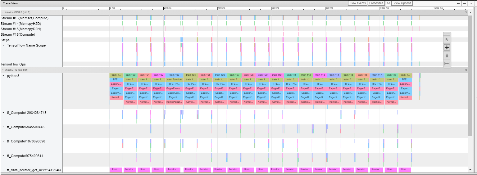
Futher analysis reveals that the GPU is inactive while the tf_data_iterator_get_next op is running on the CPU. We want to always keep the GPU active because the GPU preforms our model operations. We can either apply data augmentation as a component of our model which will then run on the GPU before the rest of the model, or we can apply data augmentation to the dataset properly so that either results are cached or the augmentation operation is buffered to run in parallel with the GPU. The latter, albeit more tricky, should provide us with optimal preformance.

data_augmentation = tf.keras.Sequential([
  layers.RandomRotation(0.05),
  layers.RandomTranslation(
      0.05,
      0.05,
      fill_mode="constant",
      fill_value=0)
])

test_dataset = prepare(X_test, y_test, batch_size=64, reshape=False, exp_dim=True, shuffle=False)
train_dataset = prepare(X_train, y_train, batch_size=64, augment=True, reshape=False, exp_dim=True)
val_dataset = prepare(X_val, y_val, batch_size=64, reshape=False, exp_dim=True)

# 4 min
val_acc = []
val_loss =[]
test_acc = []
test_loss = []
best_epoch = []


for index in (0,):

  # get model and optimiser
  adadelta_opt = tf.keras.optimizers.Adadelta(learning_rate=1, rho=0.95)
  adam_opt = tf.keras.optimizers.Adam(learning_rate=0.001)
  model = get_model_compile(adam_opt)

  # callbacks
  callbacks = []
  checkpoint = tf.keras.callbacks.ModelCheckpoint(
    f"/content/drive/My Drive/Colab Notebooks/dl_assign_2/models/cnn_aug2_model_{index}.h5",
    monitor="val_accuracy",
    verbose=0,
    save_best_only=True,
    save_weights_only=True,
    mode="max")
  tboard_callback = tf.keras.callbacks.TensorBoard(log_dir = "/content/drive/My Drive/Colab Notebooks/dl_assign_2/models/logs/",
                                                 histogram_freq = 1,
                                                 profile_batch = '100,120')
  early_stop = keras.callbacks.EarlyStopping(monitor='val_loss', min_delta=5e-4, patience=15, verbose=1)
  callbacks += [checkpoint, tboard_callback, early_stop]

  # train
  history = model.fit(train_dataset,
                    validation_data=val_dataset,
                    use_multiprocessing=True,
                    epochs = 200,
                    workers=-1,
                    callbacks=callbacks)
  
  best_model = glob.glob(f"/content/drive/My Drive/Colab Notebooks/dl_assign_2/models/cnn_aug2_model_{index}.h5")[0]

  # best epoch
  val_history = np.array(history.history['val_accuracy'])
  best_epoch.append(np.where(val_history == max(val_history))[0][0] + 1)

  # load best model
  model.load_weights(best_model)

  # best validation metrics
  loss, acc = model.evaluate(val_dataset, verbose=0)
  val_acc.append(loss)
  val_loss.append(acc)

  # best testing metrics
  loss, acc = model.evaluate(test_dataset, verbose=0)
  test_acc.append(loss)
  test_loss.append(acc)

Results¶

model_params = ((0.1, 'Adadelta', True),)
data = [x + y for x, y in zip(model_params, list(map(tuple, zip(best_epoch, val_acc, val_loss, test_acc, test_loss))))]
columns = ['Learning Rate', 'Optimiser', 'Data Augmentation', 'Best Epoch', 'Validation Loss', 'Validation Accuracy', 'Testing Loss', 'Testing Accuracy']
df_results = pd.DataFrame(data=data, columns=columns).sort_values('Validation Accuracy', ascending=False)
df_results

We now have a model with 99.38% accuracy on the test data set, which is similar to our previous result. Most importantly, the model training time has been significantly reduced. The average step time of our model training has been reduced from 54 ms to 6 ms, which is an improvement of an order of magnitude! Just by prefetching data while the GPU is running we can train our model nearly 10 times faster.

Transfer learning¶

To futher improve our model in any significant amount we need to consider transfer learning. Transfer learning often employs using large and powerful models, pretrained on general tasks which are then refined to preform specific tasks. Our images are too small to be used in most pretrained image classifiers so our images will need to be scaled up.

def change_size(image):
    img = array_to_img(image, scale=False)
    img = img.resize((84, 84))
    img = img.convert(mode='RGB')
    arr = img_to_array(img)
    return arr.astype('uint8')

data_augmentation = tf.keras.Sequential([
  layers.RandomRotation(0.1),
  layers.RandomTranslation(
      0.05,
      0.05,
      fill_mode="constant",
      fill_value=0)
])

X_train_84 = np.array([change_size(img) for img in np.expand_dims(X_train, -1)])
X_val_84 = np.array([change_size(img) for img in np.expand_dims(X_val, -1)])
X_test_84 = np.array([change_size(img) for img in np.expand_dims(X_test, -1)])

test_dataset = prepare(X_test_84, y_test, batch_size=64, reshape=False, shuffle=False)
train_dataset = prepare(X_train_84, y_train, batch_size=64, augment=True, reshape=False)
val_dataset = prepare(X_val_84, y_val, batch_size=64, reshape=False)

Add a classifier on top of Inception4 and train only the classifier¶

with tf.device('/device:GPU:0'):

  model = keras.Sequential()
  model.add(keras.applications.InceptionResNetV2(
    weights='imagenet',  
    input_shape=(84, 84, 3),
    include_top=False, 
    pooling='max'))
  # model.add(layers.Flatten())
  model.add(layers.Dense(256, activation='relu'))
  model.add(layers.BatchNormalization())
  model.add(layers.Dropout(0.4))
  model.add(layers.Dense(10, activation='softmax'))

  model.compile(optimizer=keras.optimizers.Adam(learning_rate=0.0001), loss='sparse_categorical_crossentropy', metrics=['accuracy'])

model.layers[0].trainable = False

val_acc = []
val_loss =[]
test_acc = []
test_loss = []
best_epoch = []


for index in (0,):

  # model id
  model_id = f'transformer_model_{index}'

  # callbacks
  callbacks = []
  checkpoint = get_checkpoint(model_id, weights_only=False)
  early_stop = keras.callbacks.EarlyStopping(monitor='val_loss', min_delta=5e-4, patience=5, verbose=1)
  tboard_callback = tf.keras.callbacks.TensorBoard(log_dir = "/content/drive/My Drive/Colab Notebooks/dl_assign_2/models/logs/",
                                                 histogram_freq = 1,
                                                 profile_batch = '100,120')
  callbacks += [checkpoint, tboard_callback, early_stop]

  # train model and get results
  results = train_model(model, train_dataset, val_dataset, test_dataset, 20, callbacks, model_id, verbose=1)
  val_acc.append(results[0])
  val_loss.append(results[1])
  test_acc.append(results[2])
  test_loss.append(results[3])

Results¶

model_params = ((0.0001, 'Adam', 'Inception4', True),)
data = [x + y for x, y in zip(model_params, list(map(tuple, zip(best_epoch, val_acc, val_loss, test_acc, test_loss))))]
columns = ['Learning Rate', 'Optimiser', 'Transfer Model', 'Data Augmentation', 'Best Epoch', 'Validation Loss', 'Validation Accuracy', 'Testing Loss', 'Testing Accuracy']
df_results = pd.DataFrame(data=data, columns=columns).sort_values('Validation Accuracy', ascending=False)
df_results

Train all model parameters¶

By training the entire model proformance may improve but the number of trainable parameters will increase substaintially

with tf.device('/device:GPU:0'):

  model = keras.Sequential()
  model.add(keras.applications.InceptionResNetV2(
    weights='imagenet',  
    input_shape=(84, 84, 3),
    include_top=False, 
    pooling='max'))
  model.add(layers.Dense(256, activation='relu'))
  model.add(layers.BatchNormalization())
  model.add(layers.Dropout(0.4))
  model.add(layers.Dense(10, activation='softmax'))

  model.compile(optimizer=keras.optimizers.Adam(learning_rate=0.0001), loss='sparse_categorical_crossentropy', metrics=['accuracy'])

val_acc = []
val_loss =[]
test_acc = []
test_loss = []
best_epoch = []


for index in (0,):

  # model id
  model_id = f'transformer_model_{index}'

  # callbacks
  callbacks = []
  checkpoint = get_checkpoint(model_id, weights_only=False)
  early_stop = keras.callbacks.EarlyStopping(monitor='val_loss', min_delta=5e-4, patience=5, verbose=1)
  tboard_callback = tf.keras.callbacks.TensorBoard(log_dir = "/content/drive/My Drive/Colab Notebooks/dl_assign_2/models/logs/",
                                                 histogram_freq = 1,
                                                 profile_batch = '100,120')
  callbacks += [checkpoint, tboard_callback, early_stop]

  # train model and get results
  results = train_model(model, train_dataset, val_dataset, test_dataset, 20, callbacks, model_id, verbose=1)
  val_acc.append(results[0])
  val_loss.append(results[1])
  test_acc.append(results[2])
  test_loss.append(results[3])

model_params = ((0.0001, 'Adam', 'Inception4', True),)
data = [x + y for x, y in zip(model_params, list(map(tuple, zip(best_epoch, val_acc, val_loss, test_acc, test_loss))))]
columns = ['Learning Rate', 'Optimiser', 'Transfer Model', 'Data Augmentation', 'Best Epoch', 'Validation Loss', 'Validation Accuracy', 'Testing Loss', 'Testing Accuracy']
df_results = pd.DataFrame(data=data, columns=columns).sort_values('Validation Accuracy', ascending=False)
df_results

The fine tuned model has significantly more trainable parameters (54,672,746 compared to 396,554) and as such has longer training times. Dispite the immense increase in the number of trainable parameters there is no significant increase in test set accuracy, in fact the fully trainable network lost 0.03% accuracy from 99.53% to 99.50%, but this is marginable.

Custom solutions for CIFAR10¶

Shallow Convolution Network¶

A custom basic convolution network with strong results.

def clear_variables(types={'module', 'function', 'type'}):
  class Capturing(list):
    def __enter__(self):
        self._stdout = sys.stdout
        sys.stdout = self._stringio = StringIO()
        return self
    def __exit__(self, *args):
        self.extend(self._stringio.getvalue().splitlines())
        del self._stringio
        sys.stdout = self._stdout

  with Capturing() as output:
    %whos

  variables = [(line.split()[0], line.split()[1]) for line in output[2:]]

  for var, type_ in variables:
    if not type_ in types:
      exec(f'del({var})')

(X_train, y_train) , (X_test, y_test) = keras.datasets.cifar10.load_data()
X_train, X_val, y_train, y_val = train_test_split(X_train, y_train, test_size=0.2, random_state=42)

test_dataset = prepare(X_test, y_test, batch_size=64, reshape=False, shuffle=False)
train_dataset = prepare(X_train, y_train, batch_size=64, augment=True, reshape=False)
val_dataset = prepare(X_val, y_val, batch_size=64, reshape=False)

def get_model_compile(optimizer='RMSprop'):
  with tf.device('/device:GPU:0'):
      model = keras.Sequential()
      model.add(layers.Conv2D(32, kernel_size=(3, 3), activation='relu', kernel_initializer='he_uniform', padding='same', input_shape=(32, 32, 3)))
      model.add(layers.Conv2D(32, kernel_size=(3, 3), activation='relu', kernel_initializer='he_uniform', padding='same'))
      model.add(layers.MaxPooling2D(pool_size=(2, 2)))
      model.add(layers.Conv2D(64, kernel_size=(3, 3), activation='relu', kernel_initializer='he_uniform', padding='same'))
      model.add(layers.Conv2D(64, kernel_size=(3, 3), activation='relu', kernel_initializer='he_uniform', padding='same'))
      model.add(layers.MaxPooling2D(pool_size=(2, 2)))
      model.add(layers.Conv2D(128, kernel_size=(3, 3), activation='relu', kernel_initializer='he_uniform', padding='same'))
      model.add(layers.Conv2D(128, kernel_size=(3, 3), activation='relu', kernel_initializer='he_uniform', padding='same'))
      model.add(layers.MaxPooling2D(pool_size=(2, 2)))
      model.add(layers.Flatten())
      model.add(layers.Dense(256, activation='relu'))
      model.add(layers.Dropout(0.4))
      model.add(layers.Dense(128, activation='relu'))
      model.add(layers.Dropout(0.2))
      model.add(layers.Dense(10, activation='softmax'))

      model.compile(optimizer=optimizer,
                        loss='sparse_categorical_crossentropy',
                        metrics=['accuracy'])
      
      return model

val_acc = []
val_loss =[]
test_acc = []
test_loss = []
best_epoch = []


for index in (0,):

  # model id
  model_id = f'shallow_model_{index}'

  # get model and optimiser
  adadelta_opt = tf.keras.optimizers.Adadelta(learning_rate=0.5)
  model = get_model_compile(adadelta_opt)

  # callbacks
  callbacks = []
  checkpoint = get_checkpoint(model_id)
  early_stop = keras.callbacks.EarlyStopping(monitor='val_loss', min_delta=5e-4, patience=15, verbose=1)
  callbacks += [checkpoint, early_stop]

  # train model and get results
  results = train_model(model, train_dataset, val_dataset, test_dataset, 100, callbacks, model_id, verbose=1)
  val_acc.append(results[0])
  val_loss.append(results[1])
  test_acc.append(results[2])
  test_loss.append(results[3])

model_params = ((0.5, 'Adadelta', True),)
data = [x + y for x, y in zip(model_params, list(map(tuple, zip(best_epoch, val_acc, val_loss, test_acc, test_loss))))]
columns = ['Learning Rate', 'Optimiser', 'Data Augmentation', 'Best Epoch', 'Validation Loss', 'Validation Accuracy', 'Testing Loss', 'Testing Accuracy']
df_results = pd.DataFrame(data=data, columns=columns).sort_values('Validation Accuracy', ascending=False)
df_results

The shallow covnet model has a test set misclassification of 20% which is a good result but nowhere near state of the art. A more advanced model architecture is needed for the more sophisticated dataset.

Custom Residual Network¶

A residual network employs residual blocks which skip layers in the network bringing information forward from shallow layers. This serves to counteract the vanishing gradient problem by providing hooks into early layers. A custom resnet, designed just for CIFAR10, is built below.

Model Architecture¶

def identity_block(X, filters, stage, block):
    conv_name_base = 'res' + str(stage) + block + '_branch'
    bn_name_base = 'bn' + str(stage) + block + '_branch'

    # path 1
    X_shortcut = X

    # path 2
    X = BatchNormalization(axis=3, name=bn_name_base + '2a')(X)
    X = Activation('relu')(X)
    X = Conv2D(filters=filters[0], kernel_size=(3, 3), strides=(1, 1), padding='same', name=conv_name_base + '2a', kernel_initializer=glorot_uniform(seed=0))(X)

    X = BatchNormalization(axis=3, name=bn_name_base + '2b')(X)
    # X = Dropout(0.2)(X)
    X = Activation('relu')(X)
    X = Conv2D(filters=filters[1], kernel_size=(3, 3), strides=(1, 1), padding='same', name=conv_name_base + '2b', kernel_initializer=glorot_uniform(seed=0))(X)
    

    # combine paths
    X = Add()([X, X_shortcut])
    X = Activation('relu')(X)

    return X

def conv_block(X, filters, stage, block):

    conv_name_base = 'res' + str(stage) + block + '_branch'
    bn_name_base = 'bn' + str(stage) + block + '_branch'

    # path 1
    X_shortcut = X

    # path 2

    X = BatchNormalization(axis=3, name=bn_name_base + '2a')(X)
    X = Activation('relu')(X)
    X = Conv2D(filters=filters[0], kernel_size=(3, 3), strides=(2, 2), padding='same', name=conv_name_base + '2a', kernel_initializer=glorot_uniform(seed=0))(X)

    X = BatchNormalization(axis=3, name=bn_name_base + '2b')(X)
    # X = Dropout(0.2)(X)
    X = Activation('relu')(X)
    X = Conv2D(filters=filters[1], kernel_size=(3, 3), strides=(1, 1), padding='same', name=conv_name_base + '2b', kernel_initializer=glorot_uniform(seed=0))(X)
    

    # path 1
    X_shortcut = BatchNormalization(axis=3, name=bn_name_base + '1')(X_shortcut)
    X_shortcut = Conv2D(filters=filters[0], kernel_size=(1, 1), strides=(2, 2), padding='same', name=conv_name_base + '1', kernel_initializer=glorot_uniform(seed=0))(X_shortcut)
    
    # combine paths
    X = Add()([X, X_shortcut])
    X = Activation('relu')(X)

    return X

def ResNet18(input_shape=(32, 32, 3)):

    # preliminary convolution
    X_input = Input(input_shape)
    X = BatchNormalization(axis=3, name='prelim_conv_bn')(X_input)
    X = Conv2D(filters=16, kernel_size=(3, 3), strides=(1, 1), padding='same', name='prelim_conv', kernel_initializer=glorot_uniform(seed=0))(X)

    # stage 1
    X = identity_block(X, [16, 16], stage=1, block='a')
    X = conv_block(X, [16, 16], stage=1, block='b')
    X = conv_block(X, [16, 16], stage=1, block='c')

    # stage 2
    X = identity_block(X, [16, 16], stage=2, block='a')
    X = conv_block(X, [32, 32], stage=2, block='b')
    X = conv_block(X, [32, 32], stage=2, block='c')

    # stage 3
    X = identity_block(X, [32, 32], stage=3, block='a')
    X = conv_block(X, [64, 64], stage=3, block='b')
    X = conv_block(X, [64, 64], stage=3, block='c')

    
    # pooling
    X = AveragePooling2D(pool_size=(2, 2), padding='same')(X)
    X = Flatten()(X)

    # dense layers
    X = Dense(256)(X)
    X = Activation('relu')(X)
    # X = BatchNormalization()(X)
    X = Dropout(0.4)(X)
    X = Dense(128)(X)
    X = Activation('relu')(X)

    # output
    X = Dropout(0.2)(X)
    X = Dense(10)(X)
    X = Activation('softmax')(X)

    model = Model(inputs=X_input, outputs=X, name='ResNet18')

    return model

def get_model_compile(optimizer='RMSprop'):
  with tf.device('/device:GPU:0'):
    base_model = ResNet18()
    model = Model(inputs=base_model.input, outputs=base_model.output)
    model.compile(optimizer=optimizer,
                  loss='sparse_categorical_crossentropy',
                  metrics=['accuracy'])
    
    return model

train_dataset = prepare(X_train, y_train, batch_size=64, augment=True, reshape=False)

# 3-4 min
val_acc = []
val_loss =[]
test_acc = []
test_loss = []
best_epoch = []


for index in (0,):

  # model id
  model_id = f'resnet_{index}'

  # get model and optimiser
  adadelta_opt = tf.keras.optimizers.Adadelta(learning_rate=0.5)
  model = get_model_compile(adadelta_opt)

  # callbacks
  callbacks = []
  checkpoint = get_checkpoint(model_id)
  early_stop = keras.callbacks.EarlyStopping(monitor='val_loss', min_delta=5e-4, patience=25, verbose=1)
  callbacks += [checkpoint, early_stop]

  # train model and get results
  results = train_model(model, train_dataset, val_dataset, test_dataset, 100, callbacks, model_id, verbose=1)
  val_acc.append(results[0])
  val_loss.append(results[1])
  test_acc.append(results[2])
  test_loss.append(results[3])

model_params = ((0.5, 'Adadelta', False),)
data = [x + y for x, y in zip(model_params, list(map(tuple, zip(best_epoch, val_acc, val_loss, test_acc, test_loss))))]
columns = ['Learning Rate', 'Optimiser', 'Data Augmentation', 'Best Epoch', 'Validation Loss', 'Validation Accuracy', 'Testing Loss', 'Testing Accuracy']
df_results = pd.DataFrame(data=data, columns=columns).sort_values('Validation Accuracy', ascending=False)
df_results

Cyclical Learning Rate¶

!pip install tensorflow_addons
from tensorflow_addons.optimizers import CyclicalLearningRate

# 13 min
val_acc = []
val_loss =[]
test_acc = []
test_loss = []
best_epoch = []


for index in (0,):

  # model id
  model_id = f'resnet_{index}'

  # get model and optimiser
  cyclical_learning_rate = CyclicalLearningRate(
    initial_learning_rate=5e-5,
    maximal_learning_rate=5e-3,
    step_size=800,
    scale_fn=lambda x: 1 / (1.2 ** (x - 1)),
    scale_mode='cycle')
  
  adam_opt = tf.keras.optimizers.Adam(learning_rate=cyclical_learning_rate)
  adadelta_opt = tf.keras.optimizers.Adadelta(learning_rate=0.5)
  model = get_model_compile(adam_opt)

  # callbacks
  callbacks = []
  checkpoint = get_checkpoint(model_id)
  early_stop = keras.callbacks.EarlyStopping(monitor='val_loss', min_delta=5e-4, patience=25, verbose=1)
  callbacks += [checkpoint, early_stop]

  # train model and get results
  results = train_model(model, train_dataset, val_dataset, test_dataset, 100, callbacks, model_id, verbose=1)
  val_acc.append(results[0])
  val_loss.append(results[1])
  test_acc.append(results[2])
  test_loss.append(results[3])

model_params = (('Cyclical', 'Adam', True),)
data = [x + y for x, y in zip(model_params, list(map(tuple, zip(best_epoch, val_acc, val_loss, test_acc, test_loss))))]
columns = ['Learning Rate', 'Optimiser', 'Data Augmentation', 'Best Epoch', 'Validation Loss', 'Validation Accuracy', 'Testing Loss', 'Testing Accuracy']
df_results = pd.DataFrame(data=data, columns=columns).sort_values('Validation Accuracy', ascending=False)
df_results

Performance comparison¶

The use of a cyclical learning rate allowed the model to learn much more efficiently before plateauing around a validation accuracy of 73%. The cyclical learning rate with the Adam optimiser only achieved a maximum validation accuracy of 0.7306 and a test accuracy of 72.13. This is in contrast to the Adadelta optimiser which took longer to learn (less efficient) but ultimately was able to reach a much high validation accuray of 0.7733 and test accuracy of 0.7686. Even with the same training time the adadelta optimiser outpreformed the adamm optimiser with a cyclical learning rate.

Xception Deep Dive¶

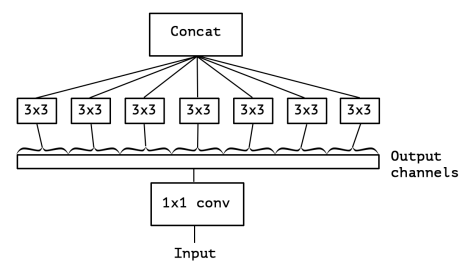
The Xception model was first introduced by Francois Chollet in 2017 on behalf of Google (Chollet, 2017). At the time the Google team had come of the back of the Inception model series, most recently having developed Inception V3, a complex CovNet architecture notable for its implementation of Inception modules in the model’s body. Inception modules consist of multiple convolutions of varying kernel sizes, canonically 1x1, 3x3, and 5x5, as well as a max pooling layer, all in parallel (Szegedy et al., 2014). These parallel layers are then concatenated into one tensor, which is then passed to the next block. This serves to increase model complexity through increased model width rather than depth, and to some degree, addresses the vanishing gradient problem.

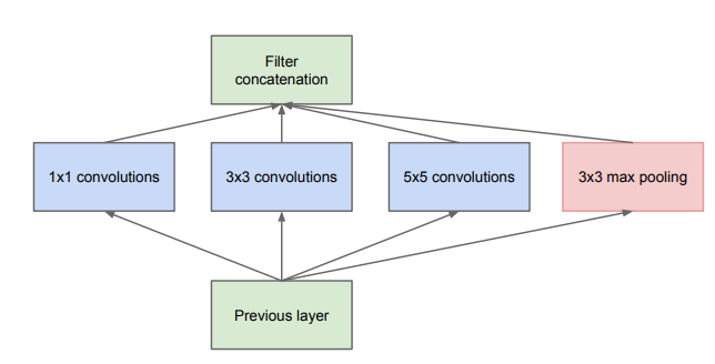
Additionally, constraints are applied to the simple inception block in order to keep the computational complexity manageable. Dimensionality reduction is achieved through the use of 1x1 kernel convolutions. Conceptually the architecture of the Inception block aims to achieve two goals, increased units per stage without runaway computational complexity, and the separation and extraction of features at different scales. The design identifies features present in different scales and combines the results. As the Inception architecture evolved so did the Inception block reaching its present form in Inception V3 shown below.

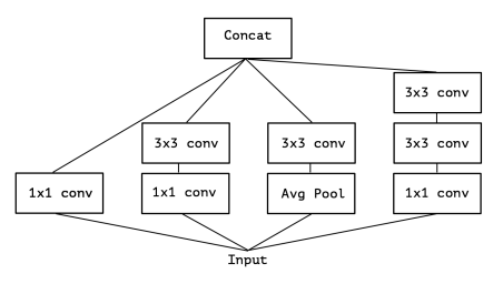
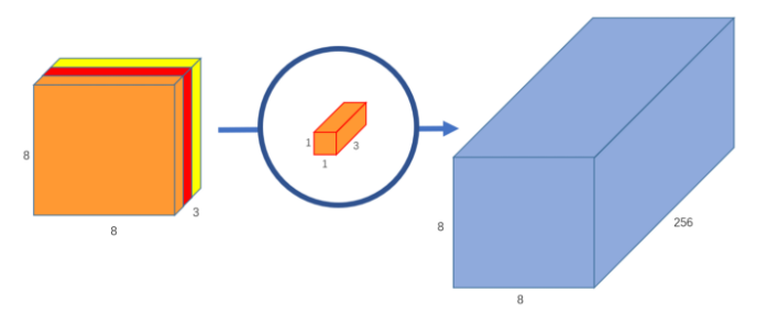
The V3 design represents a clear progression of the Inception block concept. Originally, Inception blocks identified features present in varying scales, but now they served to identify cross-channel (depth) features and spatial features separately. First, cross-channel, or depth related, relationships are captured with a pointwise convolution. These convolutions employ a 1x1 kernel which collapses depth, thus mapping depth to a single value. Several of these filters are applied to give depth.

After pointwise convolution, 3x3 or 5x5 convolutions are applied which capture spatial features. This is the essence of the Inception V3 block, obtain relationships across channels (depth) and image space (width x height), separately, one after the other, in series. Spatial features of different scales are still captured in parallel through the varying kernel size, as in the V1 design. Inception’s architecture assumes depth and spatial relationships exist, in large part, independently of each other.

Xception takes Inception to the next level by assuming depth and spatial relationship exist completely independently of each other. Following this, they should be mapped in a fully separated fashion. Xception’s body architecture consist of Xception modules, which apply pointwise convolution with as many filters as is necessary to accommodate the upcoming spatial convolution filters in a one-to-one mapping. Below, several pointwise convolution filters are applied to give many depth channels.

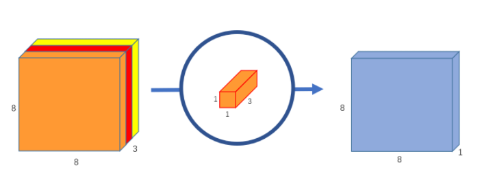
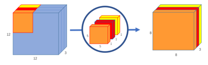
Applying each spatial convolution filter to only one depth channel constitutes what is known as depthwise convolution. This whole process allows the spatial and depth mapping to be carried out completely independently of each other. Below, depthwise convolution.

Thus, the Xception module applies pointwise convolution and depthwise convolution in series. This process is functionally equivalent to what is known as depthwise separable convolution. The only major difference being depthwise separable convolution is usually preformed in reverse, with depthwise convolution occurring before pointwise convolution. Additionally, a RELU activation is added after each step. Depthwise separable convolution was first introduced as a method of reducing model complexity (number of parameters). In a standard convolution layer with 64 filters, the tensor is transformed 64 times to a 2D plane, but with depthwise separable convolution, the tensor is transformed once during depthwise convolution and then mapped to 64 2D planes. This distinction saves an enormous amount of computation and drastically reduces the number of parameters. Below, the Xception module.

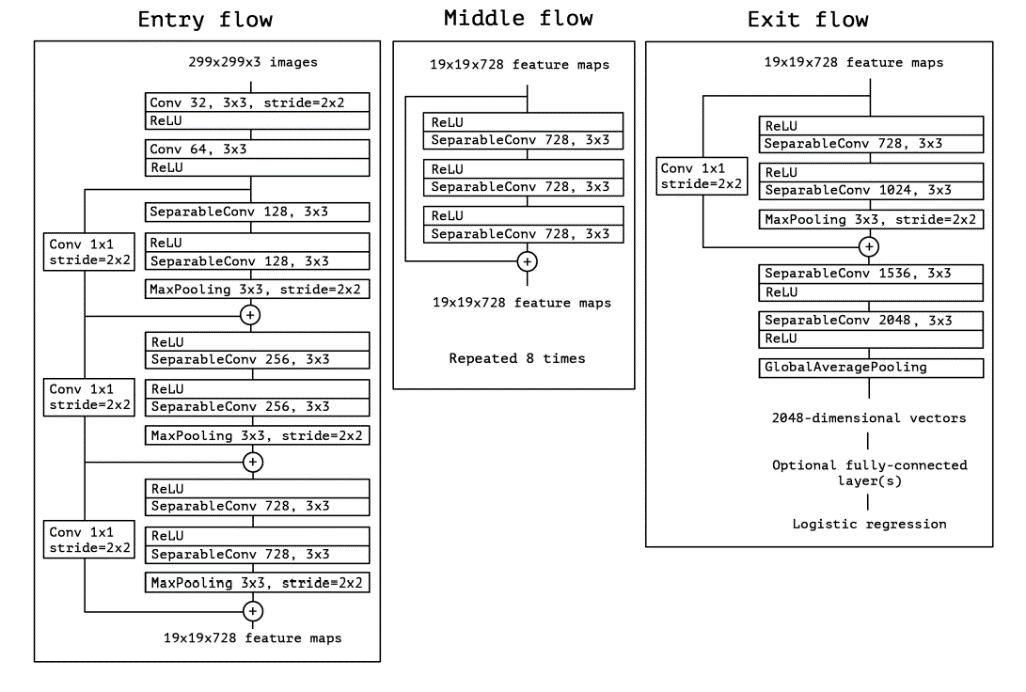
Xception modules are strung together in batches of three with a residual skip connection to form larger blocks. The canonical Xception architecture employs eight of these larger blocks in series to give the body of the model. Xception was designed for use on the ImageNet dataset (10,000 class, single-label) and the large-scale JFT dataset (17,000 class, multi-label). Thus, it has an extensive entry component, mostly consisting of blocks of two Xception modules followed by a max pooling layer. The exit component also features blocks of Xception modules and pooling layers. Below, Xception’s canonical architecture.

Xception is able to preform very well on several benchmark datasets, often scoring higher with less parameters than other much larger models. The use of depthwise separable convolution layers gives the model powerful feature extraction with fewer parameters.

Xception on CIFAR-10¶

data_augmentation = tf.keras.Sequential([
  layers.RandomRotation(0.05),
  layers.RandomTranslation(
      0.05,
      0.05,
      fill_mode="constant",
      fill_value=0)
])

(X_train, y_train) , (X_test, y_test) = keras.datasets.cifar10.load_data()
X_train, X_val, y_train, y_val = train_test_split(X_train, y_train, test_size=0.2, random_state=42)

def change_size_2(image):
    img = array_to_img(image, scale=False)
    img = img.resize((71, 71))
    img = img.convert(mode='RGB')
    arr = img_to_array(img)
    return arr.astype('uint8')

X_train_71 = np.array([change_size_2(img) for img in X_train])
X_val_71 = np.array([change_size_2(img) for img in X_val])
X_test_71 = np.array([change_size_2(img) for img in X_test])

test_dataset = prepare(X_test_71, y_test, batch_size=64, reshape=False)
train_dataset = prepare(X_train_71, y_train, batch_size=64, augment=True, reshape=False)
val_dataset = prepare(X_val_71, y_val, batch_size=64, reshape=False)

with tf.device('/device:GPU:0'):

  model = keras.Sequential()
  model.add(keras.applications.Xception(
    weights=None,  
    input_shape=(71, 71, 3),
    include_top=False, 
    pooling='max'))
  model.add(layers.Dense(256, activation='relu'))
  model.add(layers.BatchNormalization())
  model.add(layers.Dropout(0.4))
  model.add(layers.Dense(10, activation='softmax'))

  model.compile(optimizer=tf.keras.optimizers.Adadelta(learning_rate=0.9), loss='sparse_categorical_crossentropy', metrics=['accuracy'])

# 13 min
val_acc = []
val_loss =[]
test_acc = []
test_loss = []
best_epoch = []


for index in (0,):

  # model id
  model_id = f'xception_model_{index}'

  # callbacks
  callbacks = []
  checkpoint = get_checkpoint(model_id)
  early_stop = keras.callbacks.EarlyStopping(monitor='val_loss', min_delta=5e-4, patience=5, verbose=1)
  callbacks += [checkpoint, early_stop]

  # train model and get results
  results = train_model(model, train_dataset, val_dataset, test_dataset, 20, callbacks, model_id, verbose=1)
  val_acc.append(results[0])
  val_loss.append(results[1])
  test_acc.append(results[2])
  test_loss.append(results[3])

model_params = ((0.9, 'Adadelta', True),)
data = [x + y for x, y in zip(model_params, list(map(tuple, zip(best_epoch, val_acc, val_loss, test_acc, test_loss))))]
columns = ['Learning Rate', 'Optimiser', 'Data Augmentation', 'Best Epoch', 'Validation Loss', 'Validation Accuracy', 'Testing Loss', 'Testing Accuracy']
df_results = pd.DataFrame(data=data, columns=columns).sort_values('Validation Accuracy', ascending=False)
df_results

With a testing accuracy of 85.03 percent the Xception model has preformed really well. The model has fit well and retained strong generalisation. Xception definitely outpreformed both custome ResNet solutions previously examined.

References¶

Chollet, Francois. “Xception: Deep Learning with Depthwise Separable Convolutions.” 2017 IEEE Conference on Computer Vision and Pattern Recognition (CVPR), 2017, https://doi.org/10.1109/cvpr.2017.195.

Szegedy, Christian, et al. “Going Deeper with Convolutions.” 2015 IEEE Conference on Computer Vision and Pattern Recognition (CVPR), 2015, https://doi.org/10.1109/cvpr.2015.7298594.

Wang, Chi-Feng. “A Basic Introduction to Separable Convolutions.” Medium, Towards Data Science, 14 Aug. 2018, https://towardsdatascience.com/a-basic-introduction-to-separable-convolutions-b99ec3102728.

	Learning Rate	Learning Rate Schedule	Best Epoch	Validation Loss	Validation Accuracy	Testing Loss	Testing Accuracy
2	0.5	Constant	90	0.056495	0.987500	0.055915	0.9855
4	0.8	Constant	94	0.054182	0.987250	0.046508	0.9868
5	0.8	time based decay	66	0.052416	0.987167	0.049357	0.9851
0	0.1	Constant	84	0.053673	0.986000	0.049726	0.9843
3	0.5	time based decay	40	0.052665	0.985750	0.050113	0.9842
1	0.1	time based decay	96	0.057500	0.982667	0.052712	0.9830